ML Beginners Guide To Build Multi-label Fruit Identification Model

Table of Contents

1. Introduction
2. Model Building
3. Conclusion
4. Future Considerations
5. Frequently Asked Questions

Introduction

Even in the ever-changing field of agriculture, technology is still essential to maintaining the world's food supply. In this investigation, we explore the field of multi-label fruit classification, an advanced use of deep learning that holds the potential to transform the identification of several fruits in a single image.

Here, I'm creating a hands on tutorial for ML enthusiasts to create their own model from scratch. Let's start-

Model Building

1. Importing Libraries

The code starts by importing necessary Python libraries. These include standard libraries (os, shutil, glob, random, warnings), data processing libraries (numpy, pandas), visualization libraries (matplotlib, seaborn, PIL), and deep learning libraries (tensorflow, keras).

# Libraries for file and directory operations
import os
import shutil
import glob
import random

# avoid warnings
import warnings 
warnings. filterwarnings('ignore')

# Library for data processing
import numpy as np
import math
import pandas as pd

# Libraries for data visualization
import matplotlib.pyplot as plt
import matplotlib.image as mpimg
import seaborn as sns
from PIL import Image

# Libraries for deep learning model
import tensorflow as tf
from tensorflow.keras.optimizers import RMSprop,Adam
from tensorflow.keras.models import Sequential
from tensorflow.keras import layers
from keras.layers.normalization.batch_normalization import BatchNormalization
from tensorflow.keras.layers import Dense, Flatten, Conv2D
from tensorflow.keras.losses import sparse_categorical_crossentropy
from tensorflow.keras.preprocessing.image import ImageDataGenerator

2. Dataset Paths

Specifies the main path to the fruit dataset.
training_folder_path and test_folder_path: Define paths for the training and test datasets.

# dataset path
dataset_path = '/kaggle/input/fruits/fruits-360_dataset/fruits-360'

# Define training and test folders
training_folder_path = "/kaggle/input/fruits/fruits-360_dataset/fruits-360/Training"
test_folder_path = "/kaggle/input/fruits/fruits-360_dataset/fruits-360/Test"

3. Counting Labels

A function that takes a folder path and counts the number of labels (subfolders) in that directory. It uses os.walk to traverse the directory structure and counts the top-level directories.

# Counting total labels
def count_labels(folder_path):
    label_count = 0
    for _, dirs, _ in os.walk(folder_path):
        label_count += len(dirs)
        break  # Only count the top-level directories and exit the loop
    return label_count

num_labels = count_labels(training_folder_path)
print(f"Number of labels (folders) in the training dataset: {num_labels}")

4. List and Sort Labels

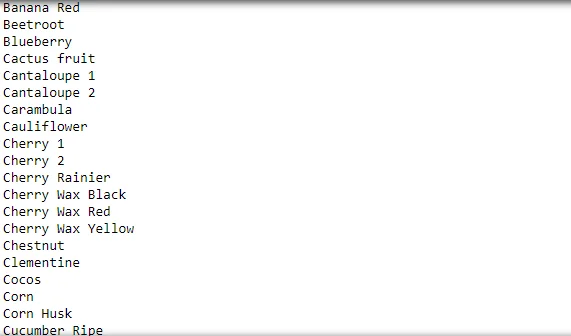
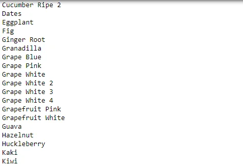
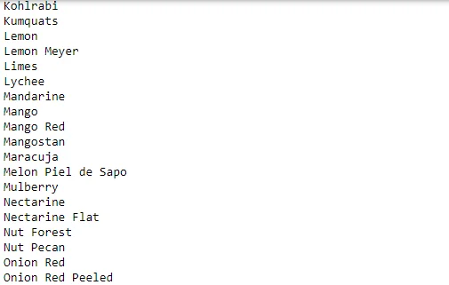
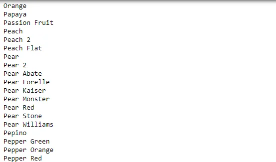
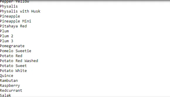
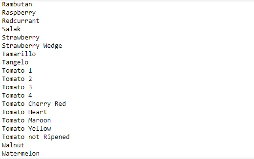
Creates a list of all labels (fruit classes) in the training dataset and sorts them alphabetically using sorted_labels.

# Get a list of all labels (subfolder names) within the training folder
labels = [label for label in os.listdir(training_folder_path) if os.path.isdir(os.path.join(training_folder_path, label))]

# Sort the labels alphabetically
sorted_labels = sorted(labels)

# Print the list of labels
print("Sorted Labels:")
for label in sorted_labels:
    print(label)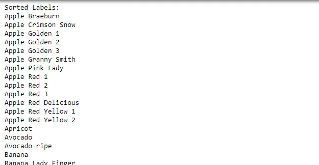

5. Creating Folders

A function to create specific folders (filtered_dataset, training, and test) in the working directory using os.makedirs.

# creating a folder for filtered dataset in the working directory

def create_folders(destination_path):
    # Create "filtered_dataset" folder directly
    os.makedirs(destination_path, exist_ok=True)

    # Create "training" and "test" folders within "filtered_dataset"
    training_path = os.path.join(destination_path, "training")
    test_path = os.path.join(destination_path, "test")
    os.makedirs(training_path, exist_ok=True)
    os.makedirs(test_path, exist_ok=True)

if __name__ == "__main__":
    destination_path = "/kaggle/working/filtered_dataset"
    create_folders(destination_path)

    print(f"filtered_dataset folder created successfully in {destination_path}")
    print(f"Training folder created successfully in {destination_path}.")
    print(f"Test folder created successfully in {destination_path}.")

6. Copy Selected Folders

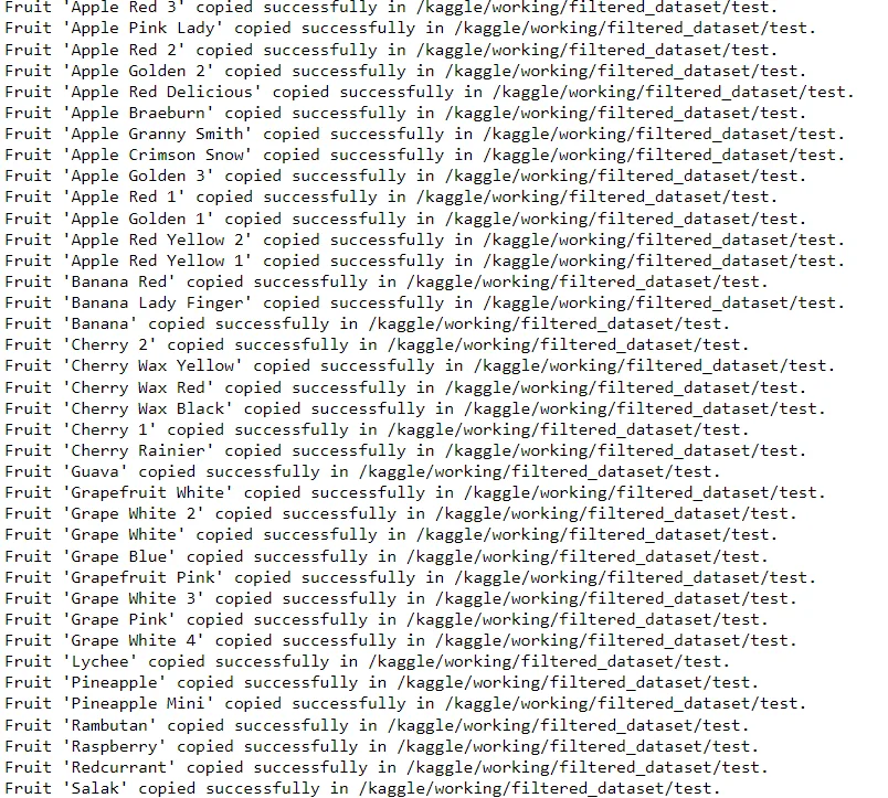
Copies selected fruit folders (e.g., Apple, Banana) from the original dataset to the filtered dataset for both training and testing. It uses shutil.copytree to copy entire folders.

def copy_selected_folders(source_path, destination_path, selected_fruits):
    if not os.path.exists(source_path):
        print("Source path does not exist.")
        return

    source_folders = os.listdir(source_path)
    for fruit_pattern in selected_fruits:
        fruit_pattern = fruit_pattern.lower()  # Make sure the fruit pattern is in lowercase
        fruit_folder_matches = [f for f in source_folders if f.lower().startswith(fruit_pattern)]

        if not fruit_folder_matches:
            print(f"No variants found for '{fruit_pattern}'.")
            continue

        for source_folder in fruit_folder_matches:
            fruit_name = source_folder
            source_folder = os.path.join(source_path, source_folder)
            destination_folder = os.path.join(destination_path, fruit_name)
            try:
                shutil.copytree(source_folder, destination_folder)
                print(f"Fruit '{fruit_name}' copied successfully in {destination_path}.")
            except FileExistsError:
                print(f"Fruit '{fruit_name}' already exists in the destination path.")
                
# copy fruit folders to training folder
if __name__ == "__main__":
    source_path = "/kaggle/input/fruits/fruits-360_dataset/fruits-360/Training"
    destination_path = "/kaggle/working/filtered_dataset/training"
    
    # Selecting the fruit names to copy all variants
    selected_fruits = ["Apple","Banana", "Cherry","Guava","Grape","Lychee","Pineapple","Rambutan","Raspberry","Redcurrant","Salak"] 
  
    copy_selected_folders(source_path, destination_path, selected_fruits)
    
# copy fruit folders to test folder
if __name__ == "__main__":
    source_path = "/kaggle/input/fruits/fruits-360_dataset/fruits-360/Test"
    destination_path = "/kaggle/working/filtered_dataset/test"
    
    # Selecting the fruit names to copy all variants
    selected_fruits = ["Apple","Banana", "Cherry","Guava","Grape","Lychee","Pineapple","Rambutan","Raspberry","Redcurrant","Salak"] 
  
    copy_selected_folders(source_path, destination_path, selected_fruits)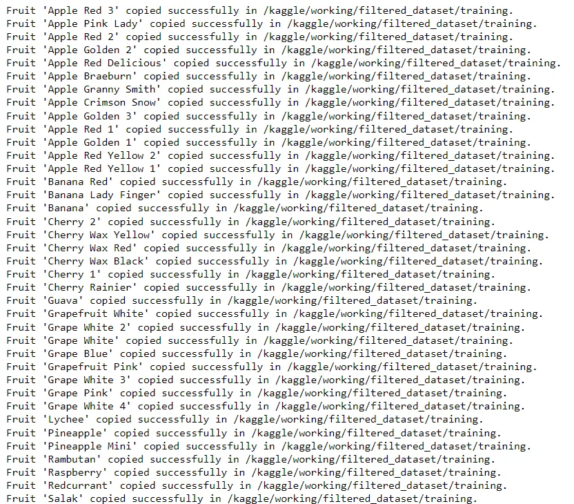

7. Counting Images per Label

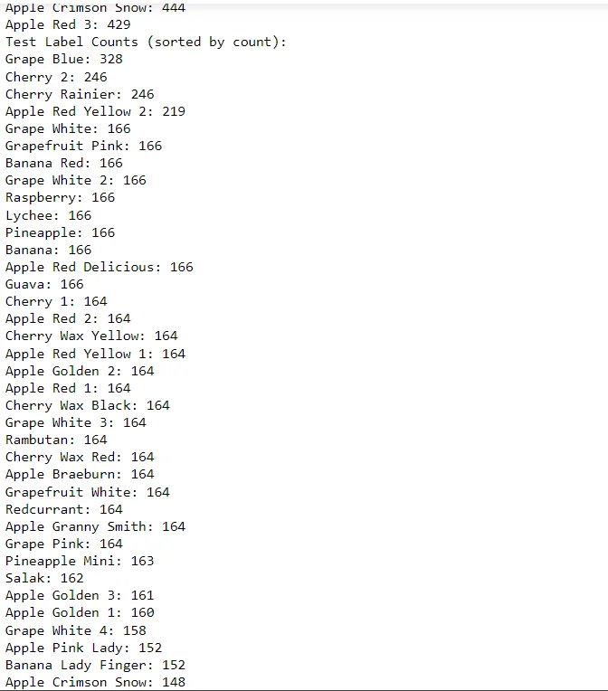
Counts the number of images for each fruit label in a given folder. It uses os.listdir and os.path.join to list files in each subfolder and counts them.

training_subset="/kaggle/working/filtered_dataset/training"
test_subset="/kaggle/working/filtered_dataset/test"

# function to count images in each folder
def count_images_per_label(folder_path):
    label_counts = {
        label: len(os.listdir(os.path.join(folder_path, label)))
        for label in os.listdir(folder_path)
        if os.path.isdir(os.path.join(folder_path, label))
    }

    return label_counts

if __name__ == "__main__":
    # Count images in training folders
    training_label_counts = count_images_per_label(training_subset)
    test_label_counts = count_images_per_label(test_subset)
    sorted_training_label_counts = sorted(training_label_counts.items(), key=lambda x: x[1], reverse=True)
    sorted_test_label_counts = sorted(test_label_counts.items(), key=lambda x: x[1], reverse=True)
print("Training Label Counts (sorted by count):")
for label, count in sorted_training_label_counts:
    print(f"{label}: {count}")
print("Test Label Counts (sorted by count):")
for label, count in sorted_test_label_counts:
    print(f"{label}: {count}")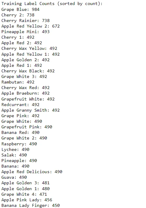

8.Counting Total Images

Counts the total number of images in a given folder using os.walk to traverse the directory structure and summing up the file counts.

#counting number of images
def count_total_images(folder_path):
    total_images = 0
    for _, _, files in os.walk(folder_path):
        total_images += len(files)
    return total_images

total_images_count = count_total_images(dataset_path)
total_train_images_count = count_total_images(training_subset)
total_test_images_count = count_total_images(test_subset)

#Display total number of images in each folder of the dataset
print(f"Total number of images in the main dataset: {total_images_count}")
print(f"Total number of images in the training dataset: {total_train_images_count}")
print(f"Total number of images in the test dataset: {total_test_images_count}")

9.Combining Label Counts

Combines and sorts label counts from the training and test datasets into a single dictionary (combined_label_counts).

# Combine the training and test label counts into a single dictionary
combined_label_counts = {
    label: training_label_counts.get(label, 0) + test_label_counts.get(label, 0)
    for label in set(list(training_label_counts.keys()) + list(test_label_counts.keys()))
}

# Create a DataFrame to hold the combined fruit counts
df_fruit_counts = pd.DataFrame({"Fruit Labels": list(combined_label_counts.keys()), "Count": list(combined_label_counts.values())})

# Sort the DataFrame by the counts in descending order
df_fruit_counts = df_fruit_counts.sort_values(by="Count", ascending=False)

10.Visualizing Top 15 Fruits

Creates a DataFrame (df_fruit_counts) to hold the combined fruit counts. It then sorts and selects the top 15 fruits based on count and plots a horizontal bar chart using Seaborn.

# Select the top 15 fruit labels by count
top_15_fruits = df_fruit_counts.head(15)

# Plot the horizontal bar chart using Seaborn
plt.figure(figsize=(10, 8))
sns.barplot(x="Count", y="Fruit Labels", data=top_15_fruits, palette="YlOrRd")
plt.xlabel("Count")
plt.ylabel("Fruit Labels")
plt.title("Top 15 Fruit Labels by Count")
plt.show()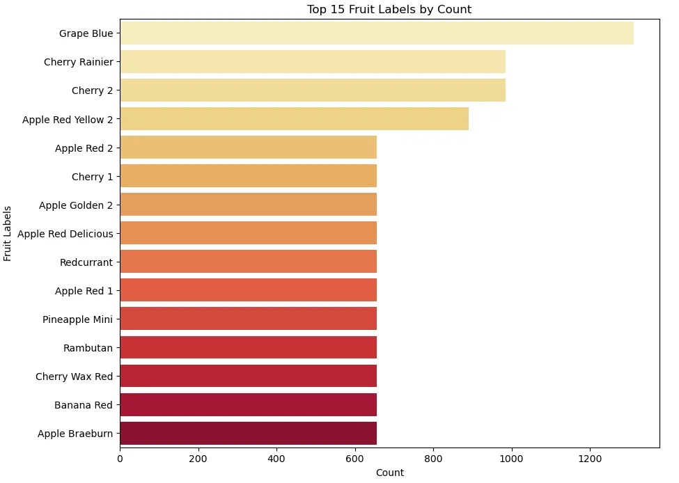

11.Data Preprocessing

Defines constants for batch size (BATCH_SIZE), image size (IMAGE_SIZE), channels (CHANNELS), and epochs (EPOCHS).

BATCH_SIZE = 32
IMAGE_SIZE = 100
CHANNELS = 3
EPOCHS = 10

12.Training Dataset Pipeline

Uses tf.keras.preprocessing.image_dataset_from_directory to create a training dataset pipeline. It performs resizing, rescaling, and shuffling of the images.

# training dataset pipeline
train_dataset = tf.keras.preprocessing.image_dataset_from_directory(
    training_subset,
    seed=42,
    shuffle=True,
    image_size=(IMAGE_SIZE,IMAGE_SIZE),
    batch_size=BATCH_SIZE
)

13.Dataset Class Names

Extracts and prints the class names from the training dataset using train_dataset.class_names.

#print training labels
tr_class_names = train_dataset.class_names
tr_class_names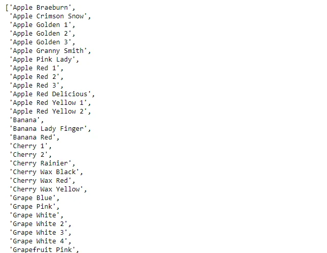

14. Visualizing Sample Images

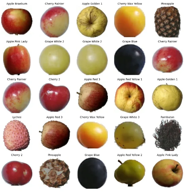
Displays a grid of sample images from the training dataset using plt.imshow and Matplotlib.

#visualizing sample images from the dataset
plt.figure(figsize=(10, 10))
for image_batch, labels_batch in train_dataset.take(9):
    for i in range(25):
        ax = plt.subplot(5,5, i + 1)
        plt.imshow(image_batch[i].numpy().astype("uint8"))
        plt.title(tr_class_names[labels_batch[i]], fontsize=10)
        plt.axis("off")

plt.tight_layout()
plt.show()

15.Dataset Splitting

get_dataset_partitions_tf: A function that takes a dataset and splits it into training and validation sets based on specified proportions.

# define a function to split the dataset 
def get_dataset_partitions_tf(ds, train_split=0.8, val_split=0.2, shuffle=True, shuffle_size=10000):
    assert (train_split + val_split) == 1

    ds_size = len(ds)

    if shuffle:
        ds = ds.shuffle(shuffle_size, seed=1234)

    train_size = int(train_split * ds_size)
    val_size = int(val_split * ds_size)

    train_ds = ds.take(train_size)
    val_ds = ds.skip(train_size).take(val_size)

    return train_ds, val_ds
    
train_ds, val_ds = get_dataset_partitions_tf(train_dataset)

#print length of each set
print("Training dataset length",len(train_ds))
print("Validation dataset length",len(val_ds))

16.Optimizing Dataset for Training:

Caching and prefetching are applied to optimize the training dataset using cache and prefetch functions.

# Optimization for Training and Validation Datasets by caching and shuffling
train_ds = train_ds.cache().shuffle(100).prefetch(buffer_size=tf.data.AUTOTUNE)
val_ds = val_ds.cache().shuffle(100).prefetch(buffer_size=tf.data.AUTOTUNE)

# resize and rescaling images to a specified size 
resize_and_rescale = tf.keras.Sequential([
  layers.experimental.preprocessing.Resizing(IMAGE_SIZE, IMAGE_SIZE),
  layers.experimental.preprocessing.Rescaling(1./255),
])

# prefetching the training data to optimize pipeline
train_ds = train_ds.prefetch(buffer_size=tf.data.AUTOTUNE)

17.Model Architecture:

Defines a Convolutional Neural Network (CNN) model using the Sequential API. It consists of convolutional layers, max-pooling layers, flattening, dense layers, and a dropout layer for regularization.

# Defining the shape of the input data batch for CNN
input_shape = (BATCH_SIZE, IMAGE_SIZE, IMAGE_SIZE, CHANNELS)

# Number of outputs
n_classes = len(tr_class_names)
n_classes

# CNN model
model = Sequential([
    resize_and_rescale,
    layers.Conv2D(32, kernel_size = (3,3), activation='relu', input_shape=input_shape),
    layers.MaxPooling2D((2, 2)),

    layers.Conv2D(32, kernel_size = (3,3), activation='relu'),
    layers.MaxPooling2D((2, 2)),
    
    layers.Conv2D(64, kernel_size =(3,3), activation='relu'),
    layers.MaxPooling2D((2, 2)),

    layers.Conv2D(64, kernel_size =(3,3), activation='relu'),
    layers.MaxPooling2D((2, 2)),

    layers.Conv2D(128, kernel_size = (3,3), activation='relu'),
    layers.MaxPooling2D((2, 2)),

    layers.Flatten(),
    layers.Dense(512, activation='relu'),
    layers.Dropout(0.25),
    layers.Dense(n_classes, activation='softmax'),
])

model.build(input_shape=input_shape)

# Review the model summary
model.summary()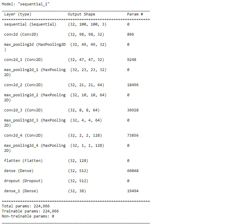

18.Compiling the Model:

Compiles the model with specified optimizer ('rmsprop'), loss function (SparseCategoricalCrossentropy), and metrics ('accuracy').

# specifying the optimizer and model metrics
model.compile(
    optimizer='rmsprop',
    loss=tf.keras.losses.SparseCategoricalCrossentropy(from_logits=True),
    metrics=['accuracy']
)

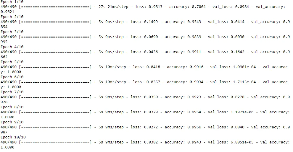
19.Model Training:

Trains the model using the training dataset and validates it using the validation dataset. The training history is stored in the history variable.

# saving the model training history
history = model.fit(
  train_ds,
  validation_data=val_ds,
  epochs=EPOCHS
)

20.Plotting Training History:

Plots the training and validation losses and accuracies over epochs using Matplotlib.

#Plotting train & validation loss
plt.figure()
plt.plot(history.history["loss"],label = "Train Loss", color = "black")
plt.plot(history.history["val_loss"],label = "Validation Loss", color = "blue", linestyle="dashed")
plt.title("Model Losses", color = "darkred", size = 15)
plt.legend()
plt.show()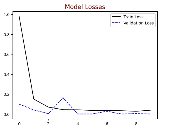

#Plotting train & validation accuracy
plt.figure()
plt.plot(history .history["accuracy"],label = "Train Accuracy", color = "black")
plt.plot(history .history["val_accuracy"],label = "Validation Accuracy", color = "blue", linestyle="dashed")
plt.title("Model Accuracy", color = "darkred", size = 15)
plt.legend()
plt.show()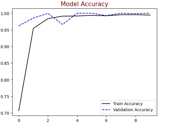

21.Test Dataset Pipeline:

Creates a test dataset pipeline using tf.keras.preprocessing.image_dataset_from_directory.

# test dataset pipeline
test_dataset = tf.keras.preprocessing.image_dataset_from_directory(
   test_subset,
    seed=42,
    shuffle=True,
    image_size=(IMAGE_SIZE,IMAGE_SIZE),
    batch_size=BATCH_SIZE
)

#print training labels
ts_class_names = test_dataset.class_names
ts_class_names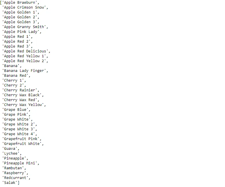

22.Fetching Model Predictions:

Displays a sample image from the test dataset along with its actual and predicted labels. Uses the model.predict function to obtain predictions.

# Fetching model predictions for sample image in test dataset
plt.figure(figsize=(3, 3))
for images_batch, labels_batch in test_dataset.take(1):

    first_image = images_batch[0].numpy().astype('uint8')
    first_label = labels_batch[0].numpy()
    print("first image to predict")
    plt.imshow(first_image)
    print("actual label:",ts_class_names[first_label])

    batch_prediction = model.predict(images_batch)
    print("predicted label:",tr_class_names[np.argmax(batch_prediction[0])])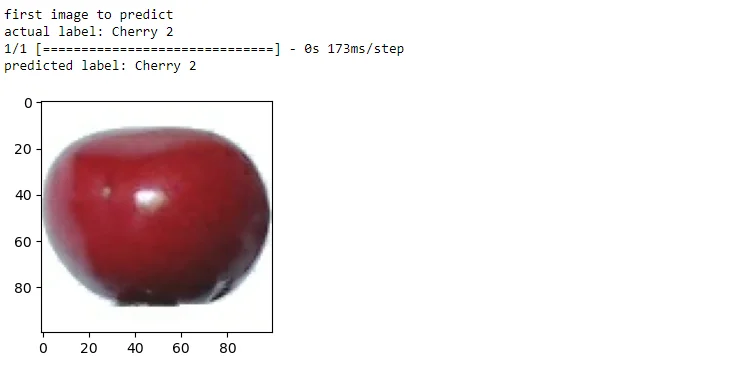	

23.Prediction Function:

Predict function that takes a model and an image and returns the predicted class and confidence percentage.

# Defining prediction function for testing images
def predict(model, img):
    img_array = tf.keras.preprocessing.image.img_to_array(images[i].numpy())
    img_array = tf.expand_dims(img_array, 0)

    predictions = model.predict(img_array)

    predicted_class = ts_class_names[np.argmax(predictions[0])]
    confidence = round(100 * (np.max(predictions[0])), 2)
    return predicted_class, confidence

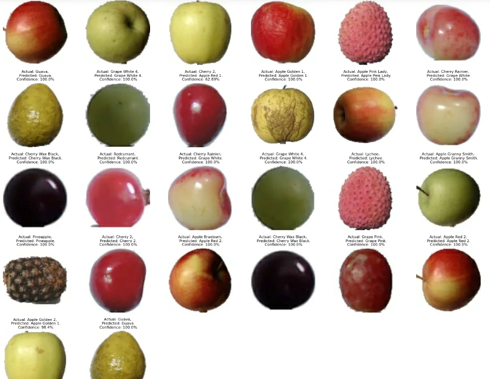
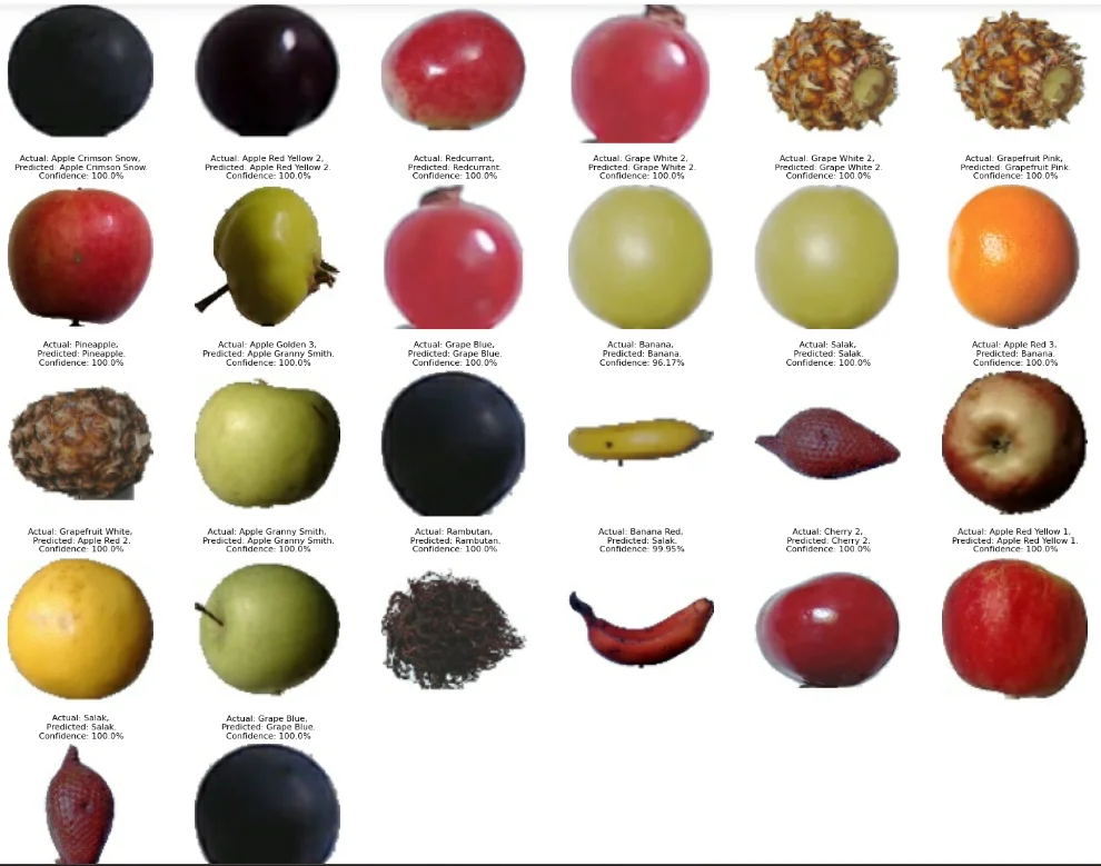
24.Visualizing Test Predictions:

Iterates over the test dataset batches and displays predictions for each image. Creates a grid of images with their actual and predicted labels.

plt.figure(figsize=(15, 15))

# Iterate over the batches and then the images to display their predictions
batch_size = 32
for images, labels in test_dataset.take(12):
    for i in range(batch_size):
        if i >= len(images):
            break

        ax = plt.subplot(6, 6, i + 1)
        image = tf.image.resize(images[i], (100, 100))
        plt.imshow(image.numpy().astype("uint8"))
        predicted_class, confidence = predict(model, images[i].numpy())
        actual_class = ts_class_names[labels[i]]
        plt.title(f"Actual: {actual_class},\n Predicted: {predicted_class}.\n Confidence: {confidence}%", fontsize=8)
        plt.axis("off")

    # If there are more than batch size images, break out of the loop
    if i >= batch_size - 1:
        break

# Hide any empty subplots
for i in range(i + 1, batch_size):
    plt.subplot(6,6, i + 1)
    plt.axis("off")

plt.tight_layout()
plt.show()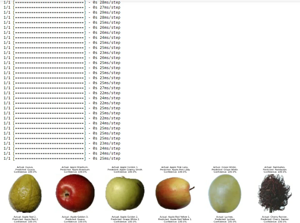

plt.figure(figsize=(15, 15))

# Iterate over the batches and then the images to display their predictions
batch_size = 32
for images, labels in test_dataset.take(15):
    for i in range(batch_size):
        if i >= len(images):
            break

        ax = plt.subplot(6, 6, i + 1)
        image = tf.image.resize(images[i], (100, 100))
        plt.imshow(image.numpy().astype("uint8"))
        predicted_class, confidence = predict(model, images[i].numpy())
        actual_class = ts_class_names[labels[i]]
        plt.title(f"Actual: {actual_class},\n Predicted: {predicted_class}.\n Confidence: {confidence}%", fontsize=8)
        plt.axis("off")

    # If there are more than batch size images, break out of the loop
    if i >= batch_size - 1:
        break

# Hide any empty subplots
for i in range(i + 1, batch_size):
    plt.subplot(6,6, i + 1)
    plt.axis("off")

plt.tight_layout()
plt.show()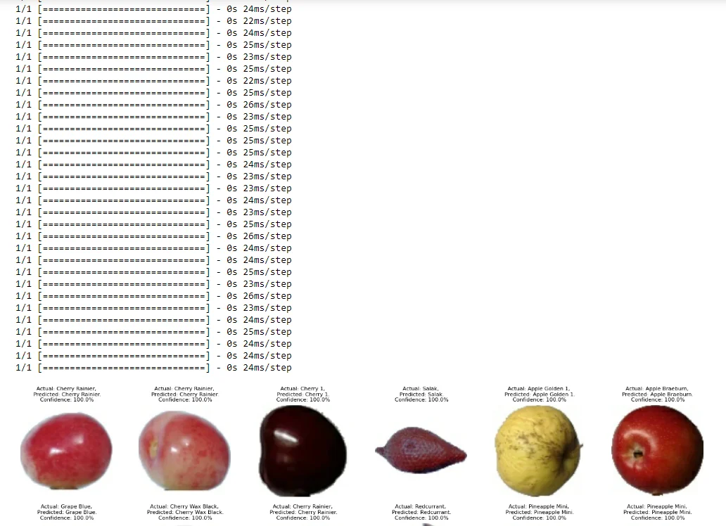

Conclusion

Finally, the exploration of multi-label fruit classification reveals an exciting new area for agriculture. Precision farming can now quickly identify a variety of fruits from a single frame thanks to the combination of deep learning and agricultural expertise.

The steps for setting up a dataset, training a CNN model, and assessing the model's effectiveness on a multilabel fruit classification job are all outlined in this script.

Future Considerations

1.Improvement through Fine-Tuning:

Constant attempts to raise the model's precision for particular fruit varieties or environmental circumstances.

2.Integration into Agricultural Systems:

Investigating how to include fruit classification models for in-the-moment monitoring and decision-making into current agricultural systems.

3.Community Participation:

Stressing the cooperative role of communities in obtaining information, validating models, and resolving local issues related to fruit classification.

Insights and resources are provided by this investigation to help agricultural stakeholders adopt multi-label fruit classification and support a robust and sustainable agricultural environment.

Frequently Asked Questions

1.What are the characteristics of multiple fruits?

A full inflorescence, such as the fig and pineapple, is represented by many fruits, which are the gynoecia of multiple flowers. Accessory fruits use additional floral components to help the mature fruit develop.

2.What are the classification of multiple fruits?

A single fruit known as a multiple or composite fruit is produced by combining all of the blooms in the entire inflorescence. Multiple fruits come in two varieties: sorosis and syconus.

3.How do you label fruit?

The correct name of the food should be written on fruit and vegetables. The majority of fruits and vegetables must be labelled with their class, and in some cases, the variety and country of origin as well. Any other descriptions should be carefully checked to make sure they are accurate.

4.How do you detect fruit quality using a sensor?

Typically, they send out an electromagnetic radiation beam—such as an infrared or laser beam—and then watch for the radiation that bounces off an item. The distance to the sensor can be determined by timing the laser beam's emission and the signal's return bounce.