Eyes of Precision- Experts Guide On Automated Casting Inspection Model Training with CNNs

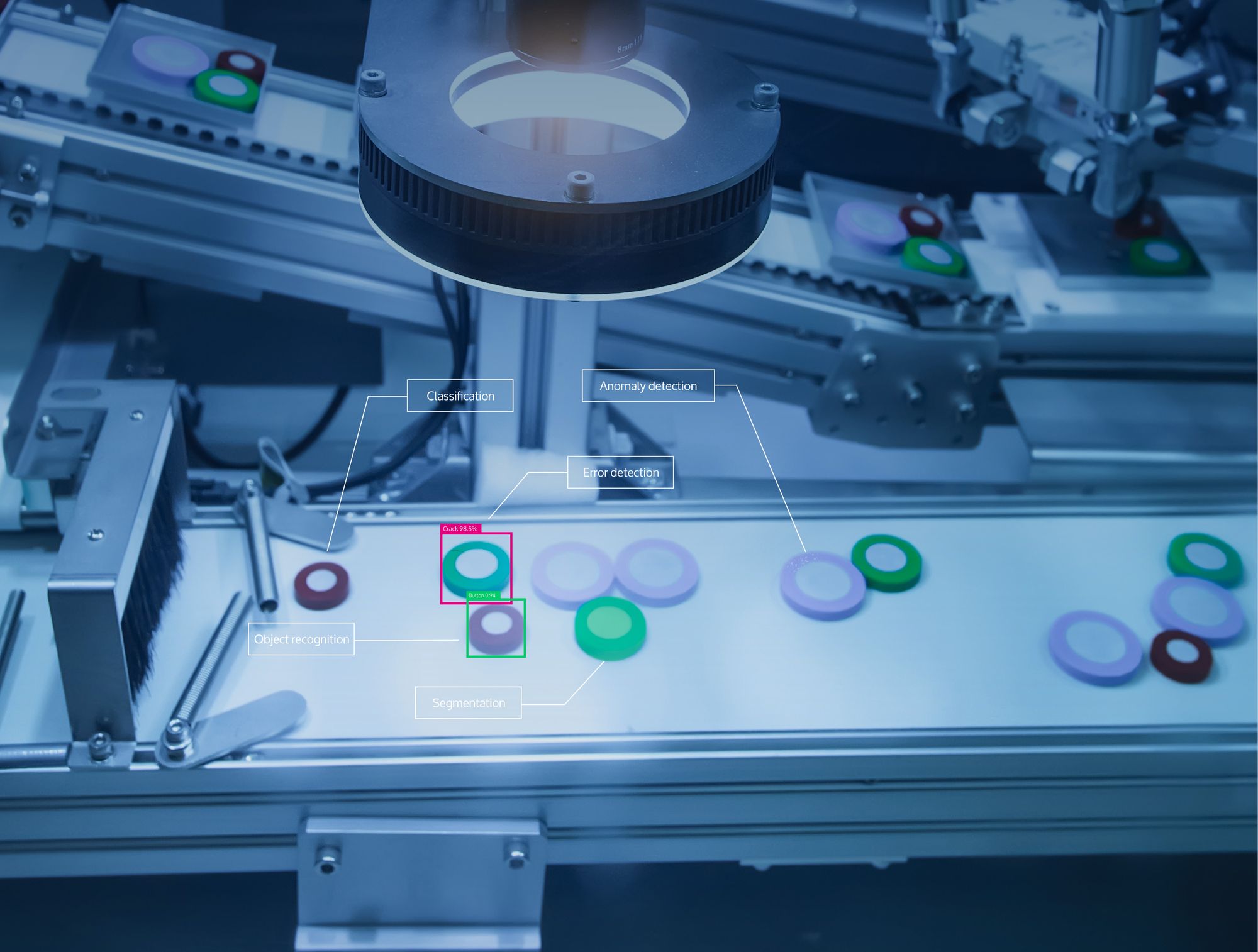
Table of Contents

1. Introduction
2. About Dataset
3. Hands-on Tutorial
4. Conclusion
5. Frequently Asked Questions

Introduction

Casting is a crucial step in the complex process of making metal products in the manufacturing industry. On the other hand, flaws and anomalies may tarnish the output, resulting in rejection and lost income. Businesses use quality inspection methods to counter this, one popular but labor-intensive approach is visual inspection. This tutorial discusses a novel way to increase productivity and accuracy, automating the visual assessment of casting products using a Convolutional Neural Network (CNN).

This tutorial is for ML researchers, product managers and data scientist who want to build a Automated Casting Inspection with CNNs .

About Dataset

The foundation of any machine learning project lies in the data. Here, we delve into the dataset provided by Pilot Technocast, containing over 7,300 top-view images of cast submersible pump impellers. The dataset is structured into training and testing sets, each further categorized into defective (def_front) and non-defective (ok_front) classes.

Hands-on Tutorial

Here are steps that we'll follow to build our model from scratch.

Outline

1.Loading and Organizing Data
2.Data Training
3.Image Visualization
4.Data Preprocessing
5.CNN Implementation
6.Training the Model
7.Model Evaluation
8.Prediction
9.Testing

1.Loading and Organizing Data

We utilize Python libraries such as Numpy,Pandas,OS,to load and organize the dataset. The images are segregated into classes, and we gain insights into the size of each class in both the training and testing data.

import os  # Operating system functionality
import random  # Random number generator
import pandas as pd  # Data analysis & manipulation
import numpy as np  # Array-processing
import seaborn as sns  # Data visualization
import matplotlib.pyplot as plt  # Data visualization
from tensorflow.keras import preprocessing, layers, models, callbacks  # Neural networks
from sklearn import metrics  # Model evaluation

2.Data Training

An essential step in model training is splitting the data into training and validation sets. We reserve 20% of the training set for validation to evaluate the model's performance during training.

# Specify paths for training and testing data
casting_dir = '/kaggle/input/real-life-industrial-dataset-of-casting-product/casting_data/casting_data/'
train_path = casting_dir + 'train/'
train_def_path = train_path + 'def_front/'
train_ok_path = train_path + 'ok_front/'
test_path = casting_dir + 'test/'
test_def_path = test_path + 'def_front/'
test_ok_path = test_path + 'ok_front/'

# Check the size of each class in both training and testing data
print('Train data, class def_front:', len(os.listdir(train_def_path)))
print('Train data, class ok_front :', len(os.listdir(train_ok_path)))
print('Test data, class def_front :', len(os.listdir(test_def_path)))
print('Test data, class ok_front  :', len(os.listdir(test_ok_path)))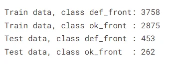

3. Image Visualization

To get a glimpse of our casting products, we visualize random images from both defective and non-defective classes. This provides an intuitive understanding of the challenges faced in visual inspection.

rand_img_def = plt.imread(
    train_def_path + random.choice(os.listdir(train_def_path)))
rand_img_ok = plt.imread(
    train_ok_path + random.choice(os.listdir(train_ok_path)))

fig, axes = plt.subplots(1, 2)
axes[0].imshow(rand_img_def, cmap='gray')
axes[1].imshow(rand_img_ok, cmap='gray')
axes[0].set_title('Defect')
axes[1].set_title('OK')
axes[0].axis('off')
axes[1].axis('off')
plt.suptitle(
    'Sample Images of Casting Product',
    y=0.9, size=16, weight='bold')
plt.show()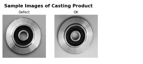

4.Data Preprocessing

A catchy segment name to describe showcasing random images, creating engagement while hinting at the neural network's visual prowess.

Before feeding our images into the hungry neural network, we preprocess them using the ImageDataGenerator. This involves rescaling pixel values to a range of 0-1, a crucial step in enhancing model convergence.

img_size, batch_size, seed_num = (300,300), 32, 0

def generate_train_img(train_path, img_size, batch_size, seed_num):
    img_generator = preprocessing.image.ImageDataGenerator(
        rescale=1./255, validation_split=0.2)
    gen_args = dict(
        target_size=img_size,
        color_mode='grayscale',
        classes={'ok_front':0, 'def_front':1},
        class_mode='binary',
        batch_size=batch_size,
        shuffle=True,
        seed=seed_num)
    train_data = img_generator.flow_from_directory(
        directory=train_path, subset='training', **gen_args)
    validation_data = img_generator.flow_from_directory(
        directory=train_path, subset='validation', **gen_args)
    return train_data, validation_data

def generate_test_img(test_path, img_size, batch_size, seed_num):
    img_generator = preprocessing.image.ImageDataGenerator(
        rescale=1./255)
    gen_args = dict(
        target_size=img_size,
        color_mode='grayscale',
        classes={'ok_front':0, 'def_front':1},
        class_mode='binary',
        batch_size=batch_size,
        shuffle=False,
        seed=seed_num)
    test_data = img_generator.flow_from_directory(
        directory=test_path, **gen_args)
    return test_data

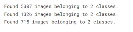
# Generate the data
train_data, validation_data = generate_train_img(
    train_path, img_size, batch_size, seed_num)
test_data = generate_test_img(
    test_path, img_size, batch_size, seed_num)

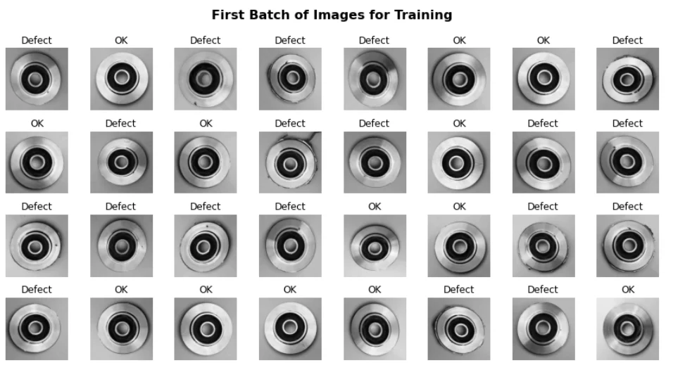
mapping_class = {0: 'OK', 1: 'Defect'}

def visualize_first_batch(dataset, fig_title):
    images, labels = next(iter(dataset))
    images = images.reshape(batch_size,*img_size)
    fig, axes = plt.subplots(4, 8, figsize=(12,6))
    for ax, img, label in zip(axes.flat, images, labels):
        ax.imshow(img, cmap='gray')
        ax.axis('off')
        ax.set_title(mapping_class[label], size=12)
    plt.tight_layout()
    fig.suptitle(fig_title, y=1.05, size=16, weight='bold')
    plt.show()
    return images

train_batch_1 = visualize_first_batch(
    train_data,
    "First Batch of Images for Training")

def visualize_pixels(selected_pxl):
    fig, ax = plt.subplots(figsize = (15,15))
    ax.imshow(selected_pxl, cmap='gray')
    ax.axis('off')
    pxl_width, pxl_height = selected_pxl.shape
    for x in range(pxl_width):
        for y in range(pxl_height):
            value = selected_pxl[x][y]
            ax.annotate(
                '{:.2f}'.format(value),
                xy=(y,x),
                ha='center',
                va='center',
                color='white' if value<0.5 else 'black')
    
visualize_pixels(selected_pxl)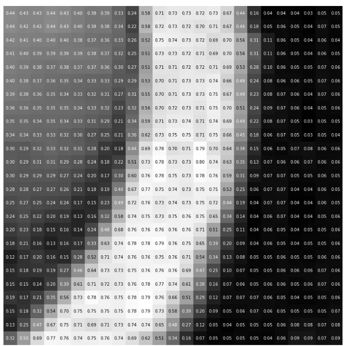

5.CNN Implementation:

We introduce a simple yet powerful CNN architecture, detailing its layers and activation functions. The model is compiled with the adam optimizer and binary crossentropy loss function, tailored for our binary classification task.

The neural network is composed of three alternating layers of MaxPooling2D and Conv2D on top of a convolutional foundation. After being flattened into a 1D shape, the final output tensors from the convolutional base are fed through two fully-connected Dense layers. The relu (rectified linear unit) activation function is used to activate the Conv2D and the first Dense layers. The addition of a Dropout layer lessens overfitting. The last Dense layer is activated by a sigmoid function that translates scores into an image's likelihood of being labelled as faulty. The Sequential constructor receives all of these layers as a list.

The model is compiled when its architecture has been defined. Utilised is the Adam Optimizer. The loss function is binary_crossentropy as the problem we are working on is binary (there are only two classes). Accuracy is the metric used to track the training.

cnn_model = models.Sequential([
    layers.Conv2D(
        filters=16,
        kernel_size=7,
        strides=2,
        activation='relu',
        padding='same',
        input_shape=img_size+(1,)),
    layers.MaxPooling2D(pool_size=2, strides=2),
    layers.Conv2D(
        filters=32,
        kernel_size=3,
        activation='relu',
        padding='same'),
    layers.MaxPooling2D(pool_size=2, strides=2),
    layers.Conv2D(
        filters=64,
        kernel_size=3,
        activation='relu',
        padding='same'),
    layers.MaxPooling2D(pool_size=2, strides=2),
    layers.Flatten(),
    layers.Dense(units=64, activation='relu'),
    layers.Dropout(rate=0.2),
    layers.Dense(units=1, activation='sigmoid')])

cnn_model.compile(
    optimizer='adam',
    loss='binary_crossentropy',
    metrics=['accuracy'])

cnn_model.summary()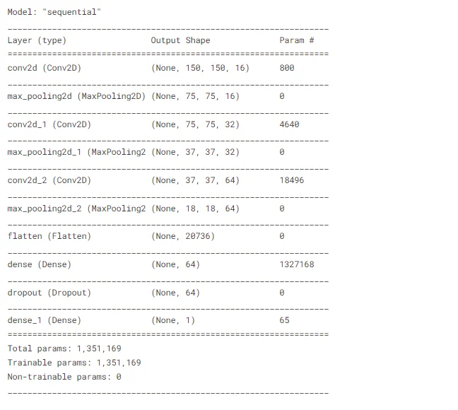

6.Training the Model:

The stage is set, and the model is ready for training. We specify the number of epochs and incorporate callbacks for early stopping and model checkpointing. The model undergoes training, with each epoch bringing us closer to a robust casting product inspector.

stop_early = callbacks.EarlyStopping(
    monitor='val_loss', patience=5)

checkpoint = callbacks.ModelCheckpoint(
    'cnn_casting_inspection.hdf5',
    verbose=1,
    save_best_only=True,
    monitor='val_loss')

n_epochs = 25

cnn_model.fit(
    train_data,
    validation_data=validation_data,
    epochs=n_epochs,
    callbacks=[stop_early, checkpoint],
    verbose=1)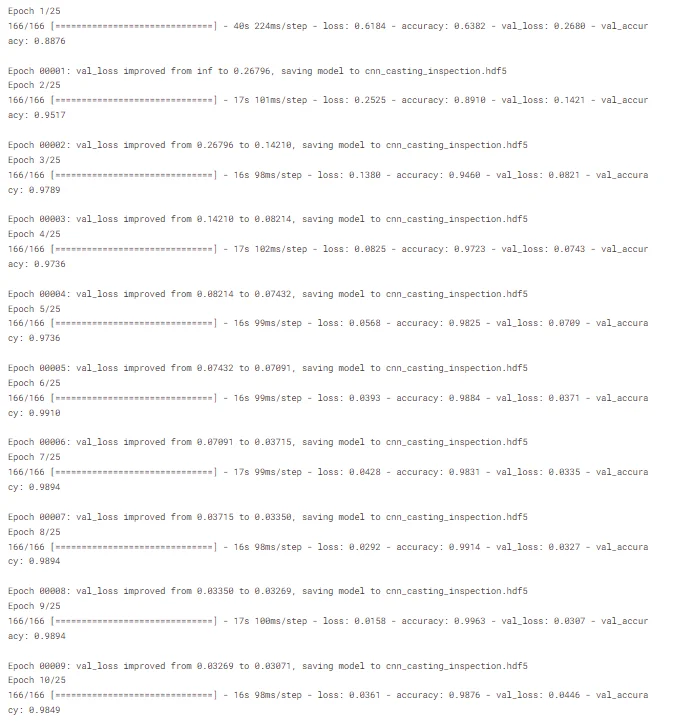

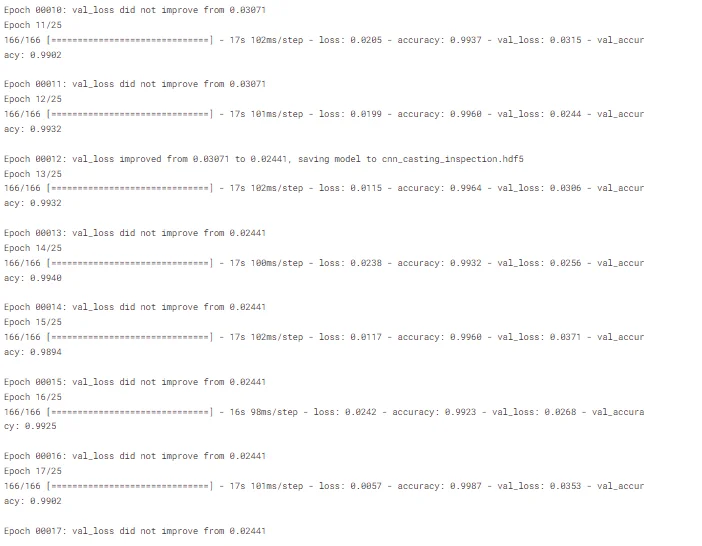
7.Model Evaluation

With 99.60% accuracy on the training set and 99.32% accuracy on the validation set, epoch 12 produces the best results. After epoch 17, training was stopped because the validation loss had not decreased from 2.44% since epoch 12. The variations in accuracy and loss on the training and validation sets are shown in the graphic below.

train_result_df = pd.DataFrame(
    cnn_model.history.history,
    index=range(1, 1+len(cnn_model.history.epoch)))

plt.subplots(figsize=(7,7))
sns.lineplot(data=train_result_df, palette='Set1')
plt.xlabel('Epochs')
plt.legend(labels=[
    'Training Loss',
    'Training Accuracy',
    'Validation Loss',
    'Validation Accuracy'])
plt.title('Model Evaluation', size=16, weight='bold')
plt.gca().spines['top'].set_visible(False)
plt.gca().spines['right'].set_visible(False)
plt.show()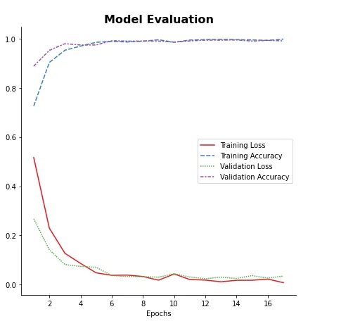

There is no indication of overfitting as the training and validation accuracies both rise with time and are closely aligned. Moreover, the losses in the validation and training sets gradually decreased to zero.

8.Prediction

Tests will be conducted to determine which model performs best in classifying photos that were excluded from the training and validation procedures. The forecast yields probability values between 0 and 1. To divide the classes, a threshold value of 0.5 has been established. A prediction probability that is equal to or greater than the threshold will be classified as Defect.

# Load the model with the best training results
best_model = models.load_model("/kaggle/working/cnn_casting_inspection.hdf5")

# Make predictions on images in the test set
y_pred_proba = best_model.predict(test_data, verbose=1)
threshold = 0.5
y_pred = y_pred_proba >= threshold

# Visualize the confusion matrix
plt.figure(figsize=(6,4))
sns.heatmap(
    metrics.confusion_matrix(test_data.classes,y_pred),
    annot=True,
    annot_kws={'size':14, 'weight':'bold'},
    fmt='d',
    xticklabels=['OK', 'Defect'],
    yticklabels=['OK', 'Defect'])
plt.tick_params(axis='both', labelsize=14)
plt.ylabel('Actual', size=14, weight='bold')
plt.xlabel('Predicted', size=14, weight='bold')
plt.show()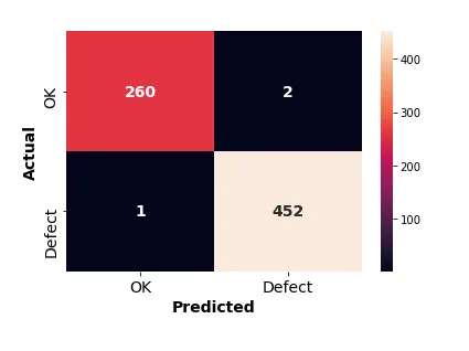

print(metrics.classification_report(
    test_data.classes, y_pred, digits = 4))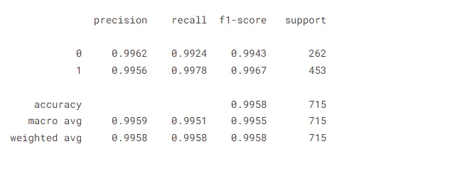

9.Testing

Visualization of the predicted outcomes on a selection of arbitrary test set photos. A comparison between the actual and anticipated class labels for each image is shown, along with the likelihood that the image belongs in the intended class.

images, labels = next(iter(test_data))
images = images.reshape(batch_size, *img_size)
fig, axes = plt.subplots(3, 4, figsize=(12,9))

for ax, img, label in zip(axes.flat, images, labels):
    ax.imshow(img, cmap='gray')
    true_label = mapping_class[label]
    [[pred_prob]] = best_model.predict(img.reshape(1, *img_size, -1))
    pred_label = mapping_class[int(pred_prob >= threshold)]
    prob_class = 100*pred_prob if pred_label == 'Defect' else 100*(1-pred_prob)
    ax.set_title(f'Actual Label: {true_label}', weight='bold')
    ax.set_xlabel(
        f'Predicted Label: {pred_label}\nProbability ({pred_label}) = {(prob_class):.2f}%',
        weight='bold', color='green' if true_label == pred_label else 'red')
    ax.set_xticks([])
    ax.set_yticks([])
    
plt.tight_layout()
fig.suptitle('Actual & Predicted Labels for Sample Test Images',
             y=1.04, size=18, weight='bold')
plt.show()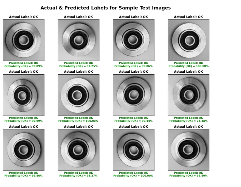

Conclusion

As the training concludes, we witness the birth of an accurate and efficient casting product inspector—a CNN model that achieved over 99.5% accuracy on the test set. The tutorial concludes with a reflection on the impact of automating visual inspection, reducing misclassifications, and paving the way for enhanced manufacturing quality.

Frequently Asked Questions

1.What is AI based visual inspection?

Ensuring that items fulfill preset requirements involves monitoring and inspecting production or service operations. Images and objects can be recorded, captured, and stored using a computer. Time is thereby saved, and efficiency is raised.

2.What is automated visual inspection?

Using cameras, image processing techniques, and machine learning algorithms, products are analyzed in real time. On-site, single-location automated visual inspections are more common than remote video inspections (RVI), in which teams transport inspection tools into the field.

3.How is AI used in quality inspection?

Product Defect Detection: Artificial intelligence (AI)-powered visual inspection automates the process of finding flaws in manufactured goods. It makes sure that only products of the highest calibre get it onto the market by identifying aesthetic problems, misalignments, poor welds, and assembly faults.