A Comprehensive Guide To Build Corrosion Detection Model For Construction Industry

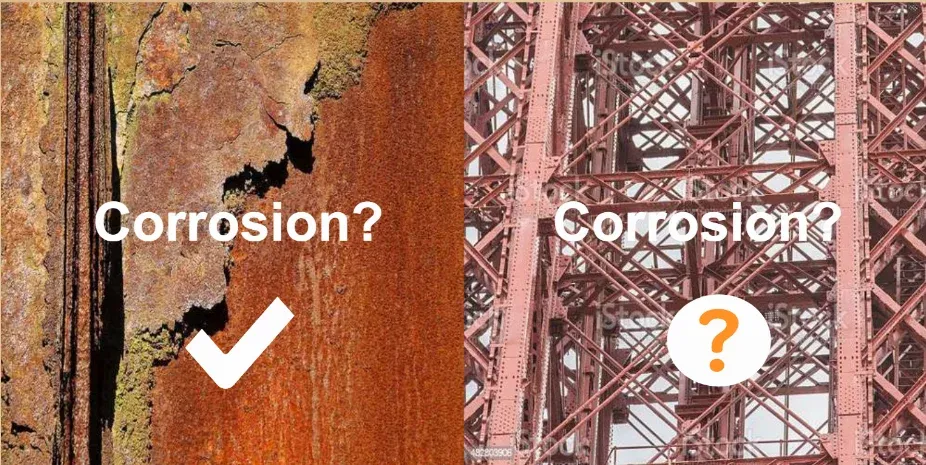
Table of Contents

1. Introduction
2. Hands-on Tutorial
3. Conclusion
4. Frequently Asked Questions

Introduction

The corrosion Environmental concerns, which cause materials to gradually deteriorate, are a constant threat to businesses ranging from manufacturing and infrastructure to oil and gas. Proactive diagnosis and management of corrosion is crucial due to its adverse effects on structural integrity. Even though they are valuable, traditional approaches are not always accurate or efficient.

A new era of corrosion detection has evolved in response to these difficulties, utilizing cutting-edge technologies to transform our understanding of and approach to combating this ubiquitous problem.

This blog explores the complexities of contemporary corrosion detection techniques and acts as a thorough guide.We'll examine the wide range of instruments changing the corrosion detection scene, from state-of-the-art imaging technologies and machine learning algorithms to cutting-edge frameworks like Gaussian Processes and UMAP (Uniform Manifold Approximation and Projection).

This tutorial is for ML researchers, product managers and data scientist who want to build a quick corrosion detection use case.

Expect to learn about a dataset that has been hand-picked for corrosion detection as well as a thorough examination of a model intended to detect surface flaws in metal.

By working together, we will unlock the promise of these cutting-edge technologies and open the door to a more sustainable and resilient future in the face of harsh obstacles. Come along on this fascinating expedition into the cutting edge of corrosion detection, where necessity meets creativity.

Hands-on Tutorial

Here are steps that we'll follow to build our model from scratch.

Outline

1.Dataset loading and directory information
2.Data Preprocessing
3.UMAP Reduction
4.Gaussian Process Classification (GPC)
5.Testing and Visualization
6.Confusion Matrix Analysis

1.Dataset loading and directory information

Incorporate the NumPy and Pandas libraries, which are frequently utilised for managing tabular data and performing numerical calculations, respectively. Additionally, import the os module to facilitate communication with the operating system.

import numpy as np
import pandas as pd
import os

import modules from the Matplotlib library for image visualization and plotting.

import matplotlib.image as mpimg 
import matplotlib.pyplot as plt

This code installs the umap-learn library using the pip package manager. UMAP (Uniform Manifold Approximation and Projection) is a dimensionality reduction technique. The library is then imported with the alias umap.

!pip install umap-learn
import umap.umap_ as umap

Import modules from the Plotly library for creating interactive plots.

import plotly.graph_objects as go
import plotly.express as px

This code installs the gpy library and imports the GPy module. GPy is a Gaussian Process (GP) framework for Python.

!pip install gpy
import GPy

import specific metrics (confusion matrix and accuracy score) from the scikit-learn library.

from sklearn.metrics import confusion_matrix, accuracy_score

installs the OpenCV library and then imports it. OpenCV is a popular computer vision library.

import cv2
!pip3 install opencv-contrib-python
!pip3 install opencv-python

This code installs the Augmentor library and imports it. Augmentor is used for image augmentation, which is a technique commonly employed in computer vision tasks to artificially increase the diversity of the training dataset.

!pip install Augmentor
import Augmentor

This line imports the shutil module, which provides a higher-level interface for file operations.

import shutil

2.Data Preprocessing

Here images of corroded and non-corroded steel surfaces are loaded and processed for further analysis. The dataset is divided into training and testing sets, and image filenames, labels, and actual images are extracted.

images_train = [];
images_test = [];
labels_train = [];
labels_test = [];
image_filenames_train = [];
image_filenames_test = [];

directory = '../input/corrosion/train'
for filename in os.listdir(directory):
    f = os.path.join(directory, filename)
    # checking if it is a file
    if os.path.isfile(f):
        #print(f)
        if f.endswith('.jpg') and ~f.endswith('a.jpg'):
            img = cv2.imread(f,0)
            images_train.append(img)  
            image_filenames_train.append(f)
            if filename.startswith('norust'):
                #print("no rust")
                labels_train.append(0)
            else:
                #print("rust")
                labels_train.append(1)

directory = '../input/corrosion/test'
for filename in os.listdir(directory):
    f = os.path.join(directory, filename)
    # checking if it is a file
    if os.path.isfile(f):
        #print(f)
        if f.endswith('.jpg') and ~f.endswith('a.jpg'):
            img = cv2.imread(f,0)
            images_test.append(img)  
            image_filenames_test.append(f)
            if filename.startswith('norust'):
                labels_test.append(0)
            else:
                labels_test.append(1)        
            
#some checks

print("images_train ", len(images_train))
print("labels_train", len(labels_train))
print("image_filenames_train", len(image_filenames_train))

print("images_test ", len(images_test))
print("labels_test", len(labels_test))
print("image_filenames_test", len(image_filenames_test))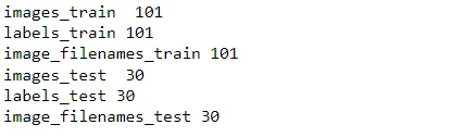

%whos

Random images from the training and testing sets are selected and displayed along with their corresponding labels. This provides a glimpse into the diversity of the dataset, showcasing both rusted and non-rusted steel surfaces.

nr_of_random_train_image = 0
print("random train image ", nr_of_random_train_image)
if labels_train[nr_of_random_train_image] == 0:
    print("NO rust")
else:
    print("Rust")
print(image_filenames_train[nr_of_random_train_image])
plt.imshow(images_train[nr_of_random_train_image])
plt.colorbar()   #Puts a color bar next to the image. 
print(type(images_train[nr_of_random_train_image]))
#print(images_train[nr_of_random_train_image])
print(images_train[nr_of_random_train_image].shape)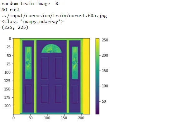

nr_of_random_test_image = 5
print("random test image ", nr_of_random_test_image)
if labels_test[nr_of_random_test_image] == 0:
    print("NO rust")
else:
    print("Rust")
print(image_filenames_train[nr_of_random_test_image])
plt.imshow(images_test[nr_of_random_test_image])
plt.colorbar()   #Puts a color bar next to the image. 
print(type(images_test[nr_of_random_test_image]))
#print(images_test[nr_of_random_train_image])
print(images_test[nr_of_random_test_image].shape)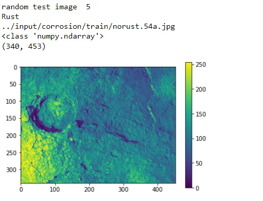

SIFT (Scale-Invariant Feature Transform) is employed to extract distinctive features from the images. Keypoints and descriptors are computed, enabling the algorithm to identify unique aspects of each image, regardless of scale or orientation.

sift = cv2.SIFT_create() #https://docs.opencv.org/4.x/da/df5/tutorial_py_sift_intro.html
kp, des = sift.detectAndCompute(images_train[nr_of_random_train_image],None)
print(des.shape)
print(des)
img=cv2.drawKeypoints(images_train[nr_of_random_train_image],kp, images_train[nr_of_random_train_image], flags=cv2.DRAW_MATCHES_FLAGS_DRAW_RICH_KEYPOINTS)
plt.imshow(img)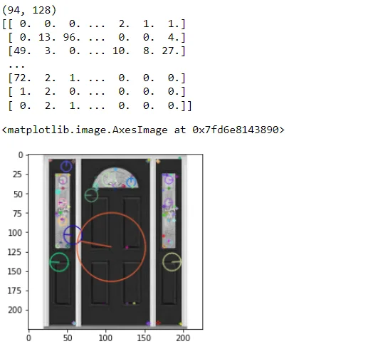

sift = cv2.SIFT_create() #https://docs.opencv.org/4.x/da/df5/tutorial_py_sift_intro.html
kp, des = sift.detectAndCompute(images_test[nr_of_random_test_image],None)
print(des.shape)
print(des)
img=cv2.drawKeypoints(images_test[nr_of_random_test_image],kp, images_test[nr_of_random_test_image], flags=cv2.DRAW_MATCHES_FLAGS_DRAW_RICH_KEYPOINTS)
plt.imshow(img)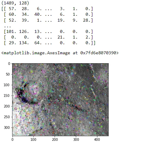

The extracted descriptors are utilized to create a Bag of Visual Words through k-means clustering. This process categorizes the features into clusters, forming a visual vocabulary that represents common patterns across the dataset.

descriptors_train_float = descriptors_train.astype(float)  

from scipy.cluster.vq import kmeans, vq
k = 128
voc, variance = kmeans(descriptors_train_float, k, 1) 

A histogram of features is generated based on the occurrences of visual words. This histogram encapsulates the image's unique characteristics, laying the foundation for subsequent analysis.

im_features_train = np.zeros((len(image_filenames_train), k), "float32")
for i in range(len(image_filenames_train)):
    words, distance = vq(des_list_train[i][1],voc)
    for w in words:
        im_features_train[i][w] += 1

The Tf-Idf vectorization is applied to further enhance feature representation. Additionally, feature scaling is performed to standardize the data, ensuring consistent and comparable results during subsequent stages.

nbr_occurences = np.sum( (im_features_train > 0) * 1, axis = 0)
idf = np.array(np.log((1.0*len(image_filenames_train)+1) / (1.0*nbr_occurences + 1)), 'float32')

from sklearn.preprocessing import StandardScaler
stdSlr = StandardScaler().fit(im_features_train)
im_features_train = stdSlr.transform(im_features_train)

im_features_train.shape

3.UMAP Reduction

UMAP is a powerful tool for gaining insights into the inherent structure of complex datasets. By projecting feature vectors into a lower-dimensional space, UMAP aids in the identification of meaningful patterns, which is crucial for subsequent stages in the corrosion detection pipeline.

In this segment, UMAP (Uniform Manifold Approximation and Projection). is introduced for dimensionality reduction. UMAP excels at capturing intricate structures in high-dimensional data, making it invaluable for revealing underlying patterns. The code initializes a UMAP reducer, specifying parameters such as the number of components and neighbors.

reducer = umap.UMAP(random_state=5,n_components=2, n_neighbors=50)
reducer.fit(im_features_train)

The UMAP reducer is applied to transform the high-dimensional feature vectors obtained from the Bag of Visual Words into a two-dimensional space. This transformation retains the essential structural information while reducing the dimensionality, facilitating visual interpretation.

embedding_train = reducer.transform(im_features_train)
assert(np.all(embedding_train == reducer.embedding_))
embedding_train.shape

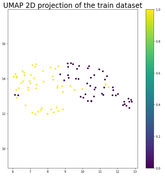
The resulting 2D UMAP projection is visualized using a scatter plot. Each point in the plot represents a metal surface image, with colors indicating the corresponding labels (corroded or non-corroded). The scatter plot provides an intuitive depiction of the relationships and groupings present in the dataset, making it easier to discern patterns and potential clusters.

plt.figure(figsize=(10,10))
plt.scatter(embedding_train[:, 0], embedding_train[:, 1], c=labels_train, s=25)
plt.gca().set_aspect('equal', 'datalim')
plt.colorbar()#boundaries=np.arange(11)-0.5).set_ticks(np.arange(10))
plt.title('UMAP 2D projection of the train dataset', fontsize=24);

4.Gaussian Process Classification (GPC)

The Gaussian Processes classifier, equipped with a sophisticated kernel and probabilistic framework, provides a robust tool for corrosion detection. By capturing uncertainties and modeling the complex relationships within the data, GP classification contributes to more informed decision-making in the corrosion analysis pipeline.

The function plot_gp is a versatile plotting utility tailored for Gaussian Process (GP) visualization. It depicts a GP fit with a 95% confidence interval, showcasing the model's uncertainty. The shaded region represents the confidence interval, while the GP mean and initial training points are illustrated.

def plot_gp(X, m, C, training_points=None):
    """ Plotting utility to plot a GP fit with 95% confidence interval """
    # Plot 95% confidence interval 
    plt.fill_between(X[:,0],
                     m[:,0] - 1.96*np.sqrt(np.diag(C)),
                     m[:,0] + 1.96*np.sqrt(np.diag(C)),
                     alpha=0.5)
    # Plot GP mean and initial training points
    plt.plot(X, m, "-")
    plt.legend(labels=["GP fit"])
    
    plt.xlabel("x"), plt.ylabel("f")
    
    # Plot training points if included
    if training_points is not None:
        X_, Y_ = training_points
        plt.plot(X_, Y_, "kx", mew=2)
        plt.legend(labels=["GP fit", "sample points"])

X = embedding_train
X.shape

y = np.array(labels_train)[:,None]
y.shape

Now establishing a GP classifier for the corrosion detection problem. The GP is configured with a Radial Basis Function (RBF) kernel and utilizes the Probit link function for Bernoulli likelihood. The Laplace approximation is employed for inference, optimizing the model for accurate predictions.

kernel = GPy.kern.RBF(2, active_dims=[0, 1], ARD=True)
probit = GPy.likelihoods.link_functions.Probit()
B_dist  = GPy.likelihoods.Bernoulli(gp_link=probit)

# We'll use Laplace approximation here
m = GPy.core.GP(  
    X, y,        
    kernel = kernel,  #  .. GP regression model used previously
    inference_method = GPy.inference.latent_function_inference.Laplace(), # Laplace approximation for inference
    likelihood = B_dist
)

m.optimize(messages=True, max_iters=200)

The GP model is trained using the provided training data (embedding_train and labels_train). Optimization is performed to fine-tune the model parameters for enhanced classification accuracy.

# Our test grid
#Xi, Xj] = np.meshgrid(np.linspace(-5,5, 100), np.linspace(-5,5, 100))
min_x = min(embedding_train[:,0])
min_y = min(embedding_train[:,1])
max_x = max(embedding_train[:,0])
max_y = max(embedding_train[:,1])
[Xi, Xj] = np.meshgrid(np.linspace(min_x-2,max_x+2, 100), np.linspace(min_y-2,max_y+2, 100))

The trained GP model is applied to a test grid (Xnew2) to make predictions.

Xnew2 = np.vstack((Xi.ravel(), Xj.ravel())).T # Change our input grid to list of coordinates

# We plot the latent function without the likelihood
#   This is equivalent to predict_noiseless in the previous lab
mean2, Cov2 = m.predict(Xnew2, include_likelihood=False, full_cov=True)


# We will also predict the median and 95% confidence intervals of the likelihood
quantiles = m.predict_quantiles(Xnew2, quantiles=np.array([50.]), likelihood=m.likelihood)
prob, _ = m.predict(Xnew2, include_likelihood=True)

The code visualizes the GP mean, variance, and 95% confidence intervals for the predicted likelihood. The left subplot illustrates the mean and median of the predicted likelihood, while the right subplot reveals the corresponding variance.

# Prepare figure environment
plt.figure(figsize=(16,6))

####
plt.subplot(121)

# # Plot the median of the predicted likelihood
plt.pcolor(Xi, Xj, prob.reshape(Xi.shape)) # (a)
plt.contour(Xi,Xj,quantiles[0].reshape(Xi.shape)) # (b)

# plt.plot(X, y, "kx", mew=2)
plt.plot(X[np.where(y == 0),0],X[np.where(y == 0),1],'bo')
plt.plot(X[np.where(y == 1),0],X[np.where(y == 1),1],'ro')

# Annotate plot
plt.xlabel("$x_1$"), plt.ylabel("$x_2$")
plt.axis("square")
plt.title("Mean")
plt.colorbar();

#====
plt.subplot(122)
# We can extract the variance from our mean function estimation of the Bernoulli distribution. 
plt.pcolor(Xi, Xj, (prob*(1.-prob)).reshape(Xi.shape)) # (c)

# Annotate plot
plt.xlabel("$x_1$"), plt.ylabel("$x_2$")
plt.title("Variance")
plt.axis("square")
plt.colorbar();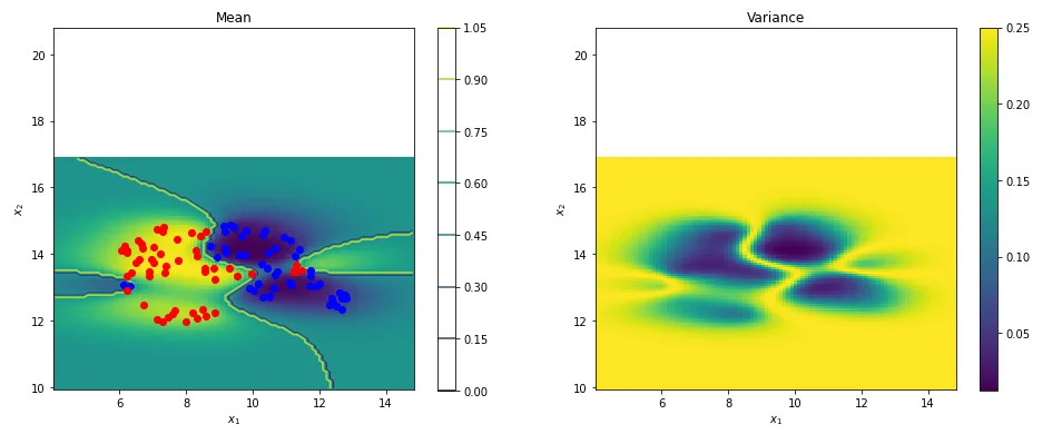

5.Testing and Visualization

The code initiates the feature extraction process for the test dataset, following the same methodology as applied to the training dataset. Key points (kp) and descriptors (des) are computed using the Scale-Invariant Feature Transform (SIFT), and the resulting descriptors are stored for further analysis.

des_list_test = [];
for i in range(len(images_test)):
    kp, des = sift.detectAndCompute(images_test[i],None)
    #print(des.shape)
    des_list_test.append((image_filenames_test[i], des)) 
descriptors_test = des_list_test[0][1];
for image_path, descriptor in des_list_test[1:]:
    descriptors_test = np.vstack((descriptors_test, descriptor))  

Test descriptors are transformed into features, and their histogram representation is calculated using the previously determined vocabulary (voc). The features are then subjected to Tf-Idf vectorization and standardized using the same scaler employed during training. The UMAP algorithm is utilized to reduce the dimensionality of the test features (embedding_test).

descriptors_test_float = descriptors_test.astype(float)  

%whos

im_features_test = np.zeros((len(image_filenames_test), k), "float32")
for i in range(len(image_filenames_test)):
    words, distance = vq(des_list_test[i][1],voc)
    for w in words:
        im_features_test[i][w] += 1

# Perform Tf-Idf vectorization
nbr_occurences = np.sum( (im_features_test > 0) * 1, axis = 0)
idf = np.array(np.log((1.0*len(image_filenames_test)+1) / (1.0*nbr_occurences + 1)), 'float32')

# Scaling the words
im_features_test = stdSlr.transform(im_features_test)

im_features_test.shape

embedding_test = reducer.transform(im_features_test)
#assert(np.all(embedding_test == reducer.embedding_))
embedding_test.shape

The reduced test features are visualized in a UMAP projection, maintaining the color-coded labels for corrosion and non-corrosion instances. This provides an insightful representation of the test dataset's structure and separation.

plt.figure(figsize=(10,10))
plt.scatter(embedding_test[:, 0], embedding_test[:, 1], c=labels_test, s=25)
plt.gca().set_aspect('equal', 'datalim')
plt.colorbar()#boundaries=np.arange(11)-0.5).set_ticks(np.arange(10))
plt.title('UMAP projection of the test dataset', fontsize=24);

The trained GP model is applied to the reduced test features (embedding_test) to make predictions. The code extracts and prints the mean predictions for the first five test instances.

X_test = embedding_test
X_test.shape

y_test = np.array(labels_test)[:,None]
y_test.shape

mean_test, Cov_test = m.predict(X_test)
print(mean_test[0:5,:])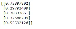

The code generates a pair of subplots for visualizing the GP classification results on the test dataset. The left subplot displays the mean and median of the predicted likelihood, while the right subplot illustrates the corresponding variance. The blue and red dots represent training instances, while blue and red 'x' markers indicate test instances with their respective corrosion labels. This visualization aids in assessing the GP model's performance on the test data.

# Prepare figure environment
plt.figure(figsize=(16,6))

####
plt.subplot(121)

# # Plot the median of the predicted likelihood
plt.pcolor(Xi, Xj, prob.reshape(Xi.shape)) # (a)
plt.contour(Xi,Xj,quantiles[0].reshape(Xi.shape)) # (b)

# plt.plot(X, y, "kx", mew=2)
plt.plot(X[np.where(y == 0),0],X[np.where(y == 0),1],'bo')
plt.plot(X[np.where(y == 1),0],X[np.where(y == 1),1],'ro')
plt.plot(X_test[np.where(y_test == 0),0],X_test[np.where(y_test == 0),1],'bx')
plt.plot(X_test[np.where(y_test == 1),0],X_test[np.where(y_test == 1),1],'rx')

# Annotate plot
plt.xlabel("$x_1$"), plt.ylabel("$x_2$")
plt.axis("square")
plt.title("Mean")
plt.colorbar();

#====
plt.subplot(122)
# We can extract the variance from our mean function estimation of the Bernoulli distribution. 
plt.pcolor(Xi, Xj, (prob*(1.-prob)).reshape(Xi.shape)) # (c)

# Annotate plot
plt.xlabel("$x_1$"), plt.ylabel("$x_2$")
plt.title("Variance")
plt.axis("square")
plt.colorbar();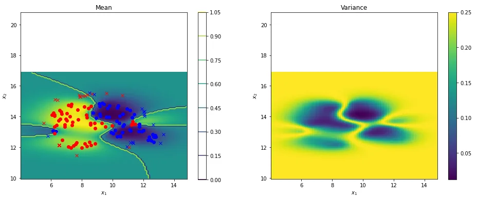

6.Confusion Matrix Analysis

Evaluation of the Gaussian Process (GP) model's performance on the test dataset. Starts by printing the mean predictions for the first five test instances to ensure the model's predictions are sensible.

print(mean_test[0:5]) #sanity check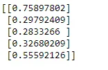

The true class labels (true_class) are compared with the predicted class labels (predictions). The code calculates the accuracy of the GP model and generates a confusion matrix to provide a comprehensive overview of the model's classification performance.

#Report true class names so they can be compared with predicted classes
true_class =  labels_test
# Perform the predictions and report predicted class names. 
predictions =  mean_test.flatten()
predictions = np.round(predictions)
predictions = predictions.astype(int)

print(true_class)
print(predictions)

A heatmap of the confusion matrix is displayed, highlighting the distribution of true positive, true negative, false positive, and false negative instances. This visual representation aids in assessing the model's strengths and weaknesses.

def showconfusionmatrix(cm):
    plt.matshow(cm)
    plt.title('Confusion matrix')
    plt.colorbar()
    plt.show()

accuracy = accuracy_score(true_class, predictions)
print ("accuracy = ", accuracy)
cm = confusion_matrix(true_class, predictions)
print (cm)

showconfusionmatrix(cm)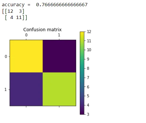

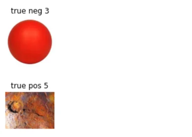
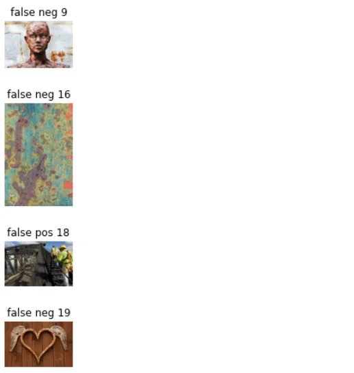
Then identifies and displays images corresponding to specific cases such as true positives, true negatives, false positives, and false negatives. This image-based analysis offers a more intuitive understanding of the model's behavior in different scenarios, contributing to a thorough evaluation of the GP model's performance on the test dataset.

import PIL
%matplotlib inline
cnt = 1;
for i in range(6):
#     print(i)
    s = ""
    if true_class[i] == 1 and predictions[i] == 1:
        s = "true pos"
    elif true_class[i] == 0 and predictions[i] == 0:
        s = "true neg"
    if s != "":
        print("nr of correctly identified ", i, " file: ", image_filenames_test[i])
        img = PIL.Image.open(image_filenames_test[i])
        plt.figure(figsize=(10, 6))
        plt.subplot(1,6,cnt)
        plt.title(s + " " + str(i))
        plt.axis('off')
        plt.imshow(img)
        cnt +=1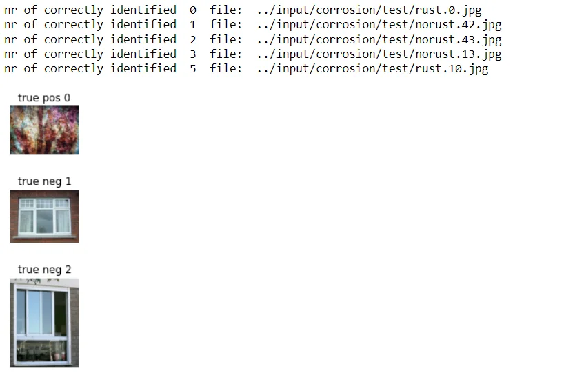

import PIL
%matplotlib inline
cnt = 1;
for i in range(len(true_class)):
#     print(i)
    s = ""
    if true_class[i] == 0 and predictions[i] == 1:
        #print("This is not rust but was mistaken as rust")
        s = "false pos"
    elif true_class[i] == 1 and predictions[i] == 0:
        #print("This is rust but was not detected as such")
        s = "false neg"
    if s != "":
        print("nr of falsely identified ", i, " file: ", image_filenames_test[i])
        img = PIL.Image.open(image_filenames_test[i])
        plt.figure(figsize=(10, 6))
        plt.subplot(2,6,cnt)
        plt.title(s + " " + str(i))
        plt.axis('off')
        plt.imshow(img)
        cnt +=1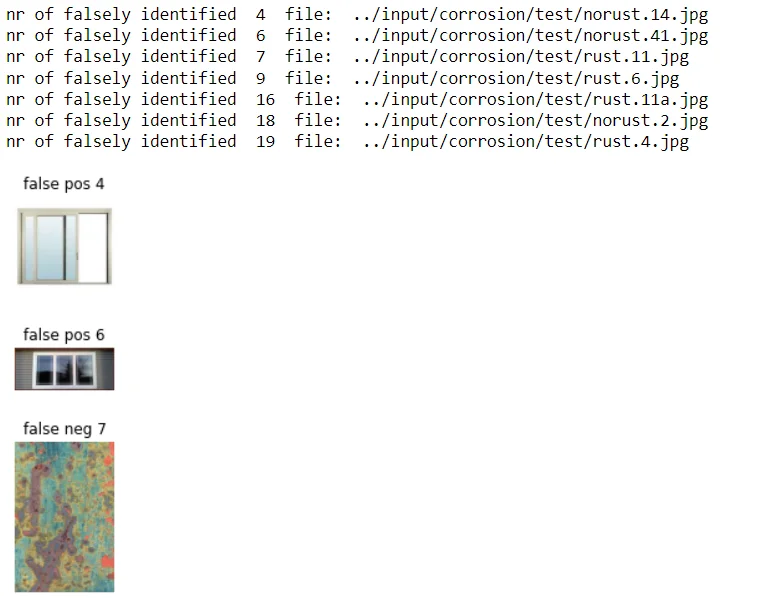

Conclusion

In summary, our investigation into the use of cutting-edge technologies for corrosion detection reveals a promising environment of efficiency and creativity. The amalgamation of state-of-the-art approaches and models, propelled by a carefully selected dataset, represents a major advancement in the ongoing battle against corrosion.

With their inherent drawbacks, traditional detection techniques are gradually being replaced by models and technologies that provide increased efficacy and accuracy.Our method, which makes use of this extensive dataset, not only overcomes the existing constraints but also gets us ready for the future requirements of corrosion detection in many industrial contexts.

Frequently Asked Questions

1.How do you detect corrosion?

Magnetic flux leakage, radiography testing, and ultrasonic testing are common NDT techniques used to find corrosion. A monitoring programme can be enhanced by additional approaches and procedures including risk-based inspection and fitness-for-service evaluations.

2.How is corrosion detected using computer vision?

In addition to other machine learning approaches like the usage of the convolutional neural network (CNN) and the genetic algorithm, corrosion detection benefits from the application of computer vision since it can recognise and classify spots of corrosion within photographs.

3.How can computer vision be used to analyze corrosion damage by spot area?

Deep learning techniques and image analysis algorithms can be applied to computer vision to analyse corrosion damage by spot area. Semantic segmentation models, such DeepLabv3, BiSeNetV2, UNET, PSPNet, and vision transformer, are one method for identifying and categorising corrosion damage.

These models use pixel-level information from the photos to precisely forecast the location and amount of corrosion. A different technique is to measure the area corroded and use computer vision algorithms to identify the different colours of corroded and non corroded surfaces.

In comparison to methods of visual analysis, this enables quantitative outputs with higher resolution.

Furthermore, the degree of corrosion in reinforced concrete structures can be estimated with the use of parameter analysis and magnetic dipole models. Combining these methods allows computer vision to analyse corrosion damage by spot area with accuracy and precision.

Looking for high quality training data to train a corrosion detection model? Talk to our team to get a tool demo.