Simple Steps To Build Security Surveillance AI Model Yourself

The security surveillance industry's problem is improving security systems' accuracy, efficiency, and scalability. This includes both hardware and software components.

Traditionally, security surveillance systems are limited by human attention and can miss crucial events or activities. Security personnel may be unable to monitor all areas at all times, leading to blind spots and potential security breaches.

Furthermore, human operators can suffer fatigue or distractions, reducing the surveillance system's effectiveness.

Enhancing security surveillance using computer vision is significant and affects many industries. While it is difficult to quantify the time and money lost due to ineffective security surveillance systems, some estimates suggest that the cost of security breaches and incidents can be substantial.

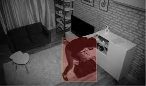
           Figure: Security Surveillance Using Computer Vision

According to a report by IBM, the average data breach cost in 2020 was $3.86 million.

This includes the direct costs of the breach, such as the cost of investigating the incident and notifying affected parties, as well as indirect costs, such as lost productivity and damage to the organization's reputation.

Computer vision plays a critical role in enhancing security surveillance systems by automating the process of monitoring and analyzing video feeds.

Using advanced computer algorithms to analyze video data, security systems can detect unusual behavior patterns or events, such as unauthorized access, theft, or vandalism.

This helps security personnel quickly identify and respond to potential threats, reducing the risk of security breaches and incidents.

Furthermore, computer vision can also reduce the workload of security personnel by enabling the automated processing and analysis of video feeds.

This allows security personnel to focus on more critical tasks, such as responding to security incidents, thereby increasing the effectiveness and efficiency of security surveillance systems.

One such company which utilizes computer vision to solve the problem of enhancing Security Surveillance Using Computer Vision is Verkada.

Verkada is a cloud-based video surveillance platform that provides enterprise-level security solutions.

Their platform allows organizations to manage and monitor their physical security systems remotely, using a web-based dashboard accessible from anywhere with an internet connection.

             Figure: Verkada's Webpage

Verkada's solution includes high-definition video cameras, access control systems, and environmental sensors, all managed and monitored through their centralized platform.

The cameras can be installed in various locations, such as offices, schools, retail stores, and manufacturing facilities, and can be configured to provide live or recorded video feeds.

Table of Contents

1. Prerequisites
2. Transfer Learning
3. Methodology
4. Dataset Selection
5. Implementation
6. Conclusion

Prerequisites

To proceed further and understand CNN based approach for detecting casting defects, one should be familiar with the following:

1. Python: All the below code will be written using python.
2. Tensorflow: TensorFlow is a free, open-source machine learning and artificial intelligence software library. It can be utilized for various tasks but is most commonly employed for deep neural network training and inference.
3. Keras: Keras is a Python interface for artificial neural networks and is open-source software. Keras serves as an interface for the TensorFlow library.
4. Kaggle: Kaggle is a platform for data science competitions where users can work on real-world problems, build their skills, and compete with other data scientists. It also provides a community for sharing and collaborating on data science projects and resources.

Apart from the above-listed tools, there are certain other theoretical concepts one should be familiar with to understand the below tutorial.

Transfer Learning

Transfer learning is a machine learning technique that adapts a pre-trained model to a new task. This technique is widely used in deep learning because it dramatically reduces the data and computing resources required to train a model.

This technique avoids the need to start the training process from scratch, as it takes advantage of the knowledge learned from solving the first problem that has already been trained on a large dataset.

The pre-trained model can be a general-purpose model trained on a large dataset like ImageNet or a specific model trained for a similar task.

The idea behind transfer learning is that the learned features in the pre-trained model are highly relevant to the new task and can be used as a starting point for fine-tuning the model on the new dataset.

Transfer learning has proven highly effective in various applications, including computer vision, natural language processing, and speech recognition.

DenseNet121

DenseNet121 is a convolutional neural network architecture introduced in 2017 as part of the DenseNet family of networks. It is a deep neural network architecture used for image classification tasks.

The "121" in the name refers to the number of layers in the network. The DenseNet121 architecture uses a dense block structure, where each layer in the network is connected to every other layer in a feed-forward manner.

This dense connectivity allows information to flow more efficiently through the network and helps to reduce the vanishing gradient problem that can occur in very deep networks.

DenseNet121 has achieved state-of-the-art performance on various image classification tasks, including the ImageNet dataset.

          Figure: DenseNet 121 Architecture

Multi-class AUC Curve

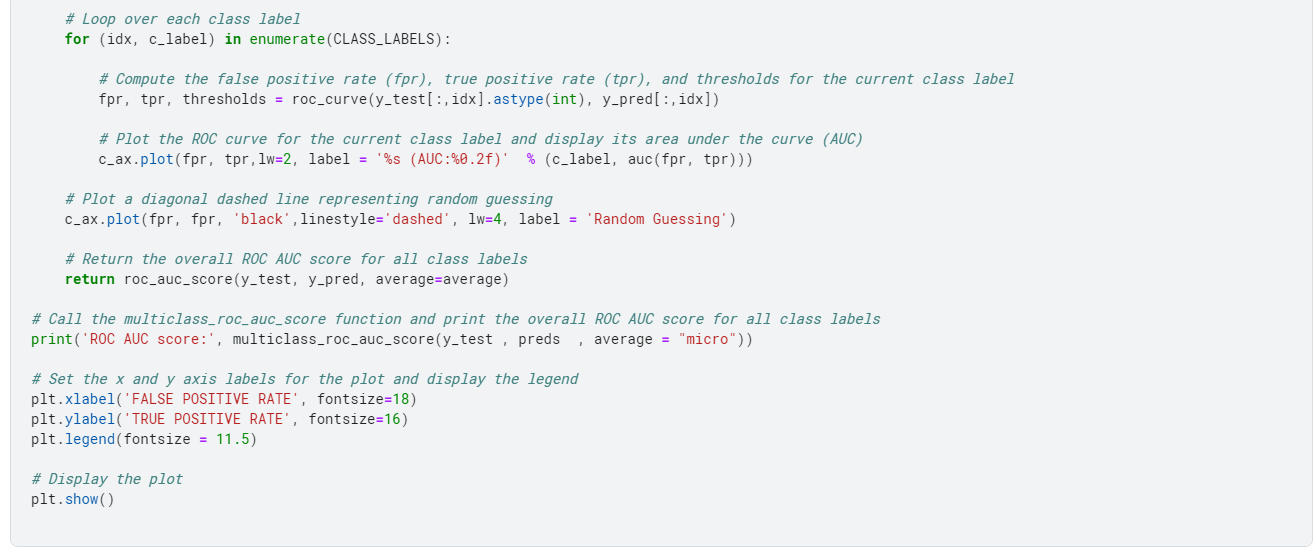
The Multi-class AUC (Area Under the Curve) Curve is a visual representation of the performance of a multi-class classification model. It plots the True Positive Rate (TPR) against the False Positive Rate (FPR) for each class label.

The TPR is the ratio of the correctly predicted positive instances to the total positive instances for a given class. The FPR is the ratio of the incorrectly predicted positive instances to the total actual negative instances for a given class.

The Multi-class AUC Curve is useful in evaluating the performance of a multi-class classification model because it shows how well the model can distinguish between different classes.

A model with a higher AUC score for a given class label indicates that it is better at distinguishing between that class and the others.

The curve provides a visual way to compare the performance of different models or algorithms for a multi-class classification problem.

The Multi-class AUC Curve can be computed by plotting the TPR against the FPR for each class label at different probability thresholds.

The curve is constructed by calculating the AUC for each class label and then averaging the AUC scores across all class labels to get a single score that represents the model's overall performance.

Methodology

To proceed with our security surveillance system, we proceed with the following steps:

1. Importing all the required libraries
2. Setting all the hyperparameters
3. Data Loading and Preprocessing
4. Feature Extraction using DenseNet121
5. Creating and Training model
6. Prediction on Test data

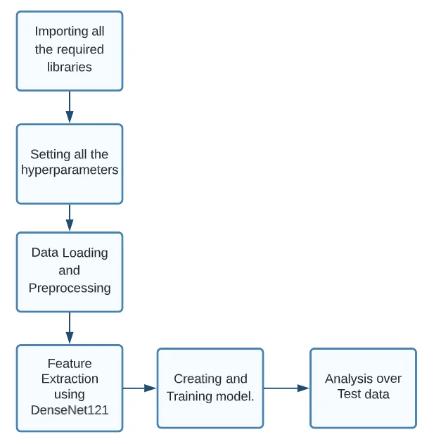
Figure: Flowchart of Methodology for Security Surveillance Using Computer Vision (Image by author)

Dataset Selection

For our above project, we used the UCF crime dataset, available on Kaggle.

The dataset contains images extracted from every video from the UCF Crime Dataset.

Every 10th frame is extracted from each full-length video and combined for every video in that class. All the images are of size 64*64 and in .png format

The dataset has a total of 14 Classes :

1. Abuse
2. Arrest
3. Arson
4. Assault
5. Burglary
6. Explosion
7. Fighting
8. Normal Videos
9. RoadAccidents
10. Robbery
11. Shooting
12. Shoplifting
13. Stealing
14. Vandalism

The total image count for the training subset is 1,266,34, while for the test subset is 111,308.

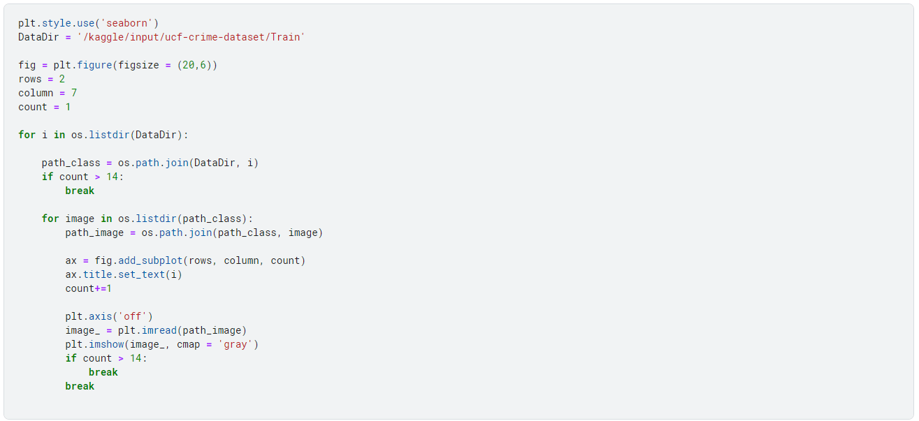
Below are some sample images from the dataset:

Implementation

Now, we begin with the coding part for security surveillance.

Environment Setup

Below are points that need to be done before running the code:

1. The below code is written in my Kaggle notebook. For this, you first need to have a Kaggle account. So, if not, you need to sign up and create a Kaggle account.
2. Once you have created your account, visit UCF Crime Dataset and create a new notebook.
3. Run the below code as given. For better results, you can try hyperparameter tuning, i.e., changing the batch size, number of epochs, etc.

Hands-on With Code

We begin by importing the required libraries.

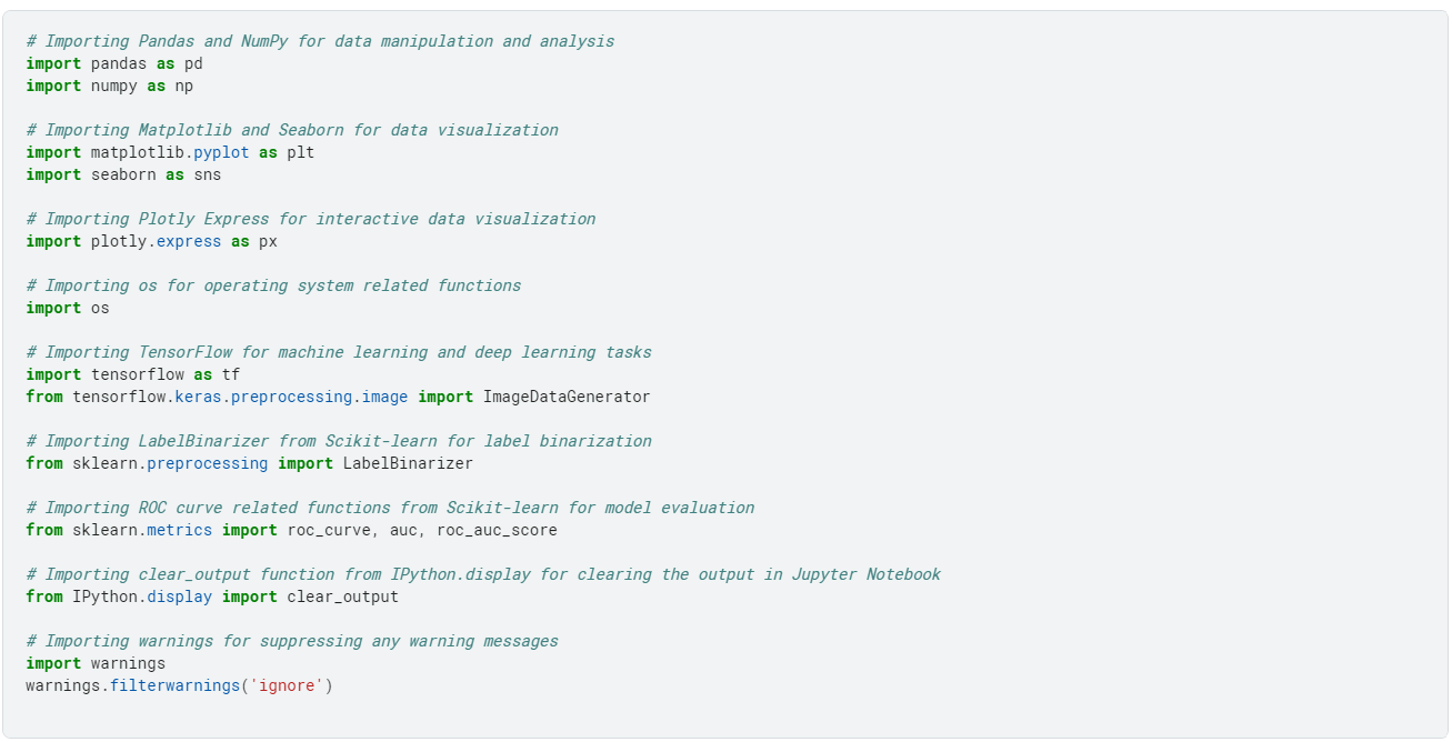
Next, we define the necessary parameters for the image dataset, which include the following:

1. Directories for the training and testing sets
2. Size of the images,
3. Batch size for training the model
4. Several epochs to train the model
5. Learning rate, the number of classes in the dataset
6. Labels for the classes.

Next, we do some data preprocessing and augmentation. For this, we use ImageGenerators, which perform real-time data augmentation.

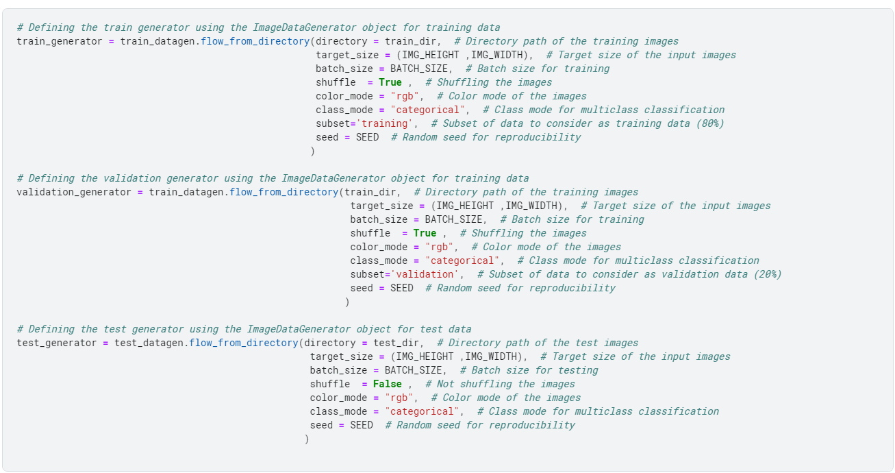
Above, we had done some data augmentation and preprocessing.

Here, the train_generator object is defined using the flow_from_directory method of the train_datagen object.

This method generates batches of images from the directory path of the training images with a target size of (64, 64), batch size of 64, shuffles the images, and converts the class labels into categorical form.

Additionally, it considers only 80% of the data as training data using the subset parameter.

The validation_generator object is also defined using the flow_from_directory method of the train_datagen object with similar parameters.

However, it considers only 20% of the data as validation data using the subset parameter.

Finally, the test_generator object is defined using the flow_from_directory method of the test_datagen object.

This method generates batches of images from the directory path of the test images with a target size of (64, 64), batch size of 64 and converts the class labels into categorical form.

However, it does not shuffle the images, as we want to predict the results in a fixed order.

For some data analysis, we look at the data distribution. We do this to check if any skewness exists within the dataset.

Why do we analyze skewness in the dataset?

Skewness is a measure of the asymmetry of a probability distribution. When a dataset is skewed, the data distribution is not symmetrical, and there is a greater concentration of values on one side of the distribution than the other.

Skewed data can lead to biased estimates of the central tendency and variability of the data, which can impact the accuracy of statistical analyses and machine learning models.

In addition, many statistical methods and machine learning algorithms assume that the data is normally distributed and can be problematic when applied to skewed data.

Therefore, it is important to identify and correct skewness in a dataset before using it for analysis or modeling.

Next, we move on to creating our model. For this, we use transfer learning. We use a pre-trained DenseNet121 model, which acts as a base model.

Why did we use DenseNet121 Model?

One reason why DenseNet121 is preferred is that it has high accuracy in image classification tasks while using fewer parameters than other popular architectures like VGG16 and ResNet50.

This makes it more efficient in terms of memory usage and Training time. Another advantage of DenseNet121 is its dense connectivity pattern, which gives each layer direct access to the gradients from the preceding layers.

This makes it easier for the network to propagate gradients during Training, leading to faster convergence and better performance.

We only change the topmost layer of this model, which takes part in the training process.

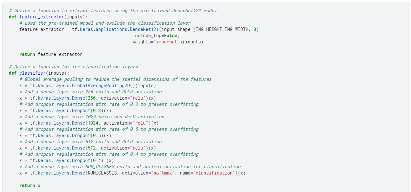
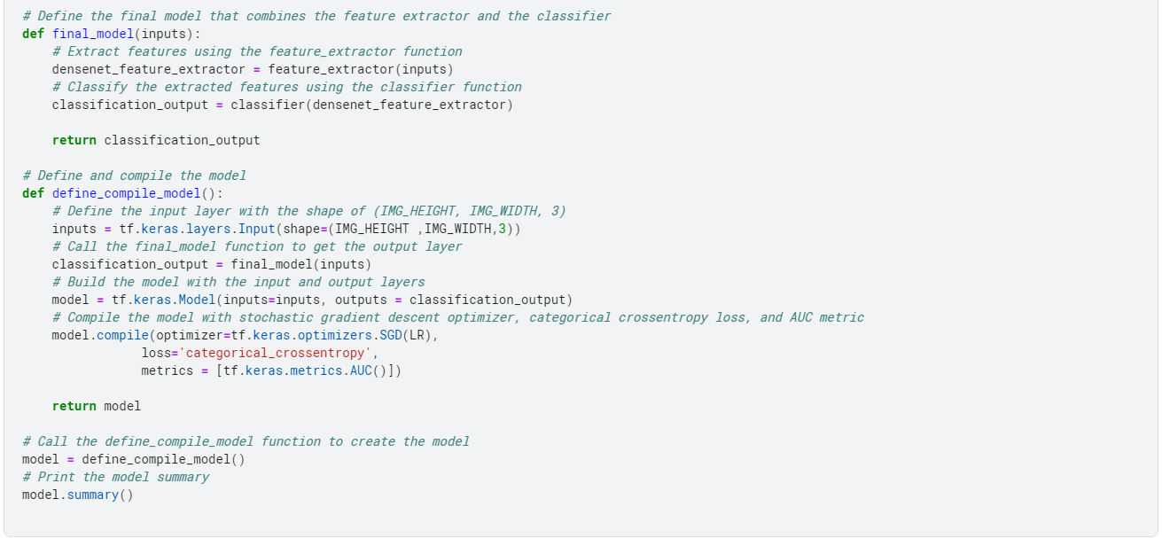
The code above defines a convolutional neural network model for image classification using the DenseNet121 architecture.

The model consists of a feature extractor, implemented using the pre-trained DenseNet121 model, and a classifier consisting of several dense layers with dropout regularization.

The model is compiled with a stochastic gradient descent optimizer, categorical cross-entropy loss, and area under the curve (AUC) metric.

The final model is defined by combining the feature extractor and classifier and is returned by the define_compile_model function.

The model summary shows the model's architecture, including the number of parameters in each layer and the output shape of each layer.

Next, we train the model.

Finally, we evaluate the performance of our model on our test data.

Conclusion

This hands-on tutorial explored the importance of computer vision enhancing security surveillance systems. Traditional security systems are limited by human attention and can miss crucial events or activities, leading to potential security breaches.

We discussed how computer vision could automate the process of monitoring and analyzing video feeds, thereby reducing the risk of security breaches and incidents.

We focused on Verkada, a cloud-based video surveillance platform that provides enterprise-level security solutions, as an example of a company utilizing computer vision to enhance security surveillance.

Their platform includes high-definition video cameras, access control systems, and environmental sensors, all managed and monitored through their centralized platform.

Furthermore, we discussed the prerequisites needed to proceed further and understand the CNN-based approach for detecting casting defects.

These include knowledge of Python, TensorFlow, Keras, and Kaggle, along with the theoretical concepts of transfer learning and DenseNet121.

Lastly, we learned about the Multi-class AUC (Area Under the Curve) Curve, a visual representation of the performance of a multi-class classification model.

It is helpful in evaluating the performance of a multi-class classification model as it shows how well the model can distinguish between different classes.