ML Guide on Cell Segmentation Using Watershed Algorithm

Introduction

Cell segmentation plays a significant role in various fields within biotechnology and life sciences, enabling researchers to analyze cellular structures and functions with precision.

One prominent technique employed for this purpose is the Watershed Algorithm, known for its effectiveness in segmenting and separating interlinked clusters within images.

The Watershed Algorithm (or one of its many variants) is a popular technique commonly used to segment & separate interlinked clusters.

Its working principle involves spreading regions out from "seed" areas (called basins), and growing these regions until they eventually touch.

The point of intersection is then taken to be the boundary between the two segmented regions (referred to as the watershed).

In this hands-on tutorial, we delve into the methodology of employing the Watershed Algorithm for segmenting red blood cells, offering a comprehensive pipeline for image processing and analysis.

Significance of Cell Segmentation

Accurate cell segmentation is crucial for advancing research in biotechnology and life sciences.

It allows scientists to study cell morphology, understand cellular interactions, and explore the intricacies of biological processes.

The segmentation of red blood cells, in particular, holds significance in medical diagnostics and research, contributing to advancements in disease detection and treatment.

Blog's Relevance

This blog serves as a valuable resource for machine learning (ML) experts, researchers, product managers, and biotechnologists seeking to enhance their understanding and application of the Watershed Algorithm in cell segmentation.

The hands-on tutorial provides a step-by-step approach, integrating machine learning techniques, color correction strategies, and parallel processing for efficient segmentation of red blood cells.

Usefulness for ML Experts

For machine learning experts, the blog offers insights into the practical implementation of the Watershed Algorithm in image segmentation.
It covers topics such as pixel classification, color correction, and evaluation metrics, providing a practical guide for leveraging ML techniques in the context of cell segmentation.

Usefulness for ML Researchers

ML researchers can benefit from the detailed methodology presented in the blog, gaining a deeper understanding of how the Watershed Algorithm can be applied to real-world challenges in cell segmentation.

The inclusion of parallel processing techniques and evaluation metrics adds a layer of sophistication, encouraging researchers to explore further advancements in the field.

Usefulness for Product Managers

Product managers in biotechnology or imaging-related industries can find valuable insights into the technical aspects of cell segmentation.
The tutorial guides them through the process, helping them make informed decisions regarding the integration of such algorithms into products and solutions.

Usefulness for Biotechnologists

Biotechnologists seeking practical applications of image segmentation will find this blog beneficial. It offers a hands-on approach to segmenting red blood cells, facilitating a deeper understanding of the underlying processes and encouraging the integration of advanced algorithms into their research workflows.

This blog provides a comprehensive and practical guide for leveraging the Watershed Algorithm in cell segmentation, catering to a diverse audience within the realms of machine learning, biotechnology, and life sciences.

Methodology

In this hands-on code approach, red-blood cells will be segmented using the watershed algorithm to produce bounding boxes. The following pipeline is deployed:

1. Image RGB to HSV conversion
2. Creating a Hue based Naive Bayes Classifier(NBC) for the pixels (2 classes - Red Blood Cells and non-Red Blood Cells)
3. Chroma-Correction on images to align their color distributions with the statistical mean of each class
4. Classifying each image pixel using the previous NBC
5. Filling of small holes produced by misclassified red-blood cell nuclei within the classification mask
6. Calculating the distance transform to closest non-RBC pixel & taking local-maxima to be the watershed basins.
7. Performing Cell Segmentation using OpenCV's Watershed Solver

Hands-on Tutorial

1. Importing Libraries

Import necessary libraries for data manipulation, visualization, and TensorFlow for deep learning.

import numpy as np # linear algebra
import pandas as pd # data processing, CSV file I/O (e.g. pd.read_csv)
import os
import os.path
import cv2 as cv
import matplotlib.pyplot as plt

# Input data files are available in the read-only "../input/" directory
# For example, running this (by clicking run or pressing Shift+Enter) will list all files under the input directory

2. Retrieving Image Paths

It traverses the '/kaggle/input' directory and collects file paths of images with the '.png' extension.

imagePathList = []

for dirname, _, filenames in os.walk('/kaggle/input'):
    for filename in filenames:
        strPath = os.path.join(dirname, filename)
        ext = os.path.splitext(filename)[1]
        if ext == '.png':
            imagePathList.append(strPath)      

3. Loading Images into HSV Color Space

Converts each image to the HSV color space using OpenCV and stores them in a dictionary (imgDict).

#dict<filename:string, hsvImage:image>
imgDict = {os.path.basename(path): cv.cvtColor(cv.imread(path), cv.COLOR_BGR2HSV) for path in imagePathList}

4. Reading Annotations from CSV

Reads the CSV file containing annotations for bounding boxes and prints the first few rows of the DataFrame.

from collections import namedtuple
from collections import defaultdict

annotationDf = pd.read_csv('/kaggle/input/blood-cell-detection-dataset/annotations.csv');
print(annotationDf.head())

5. Creating Bounding Box Labels

Defines a named tuple CellLabel for bounding box information and populates a dictionary (imgLabelDict) with image filenames and corresponding lists of bounding boxes.

#type = ['rbc'|'wbc']
CellLabel = namedtuple('CellLabel', ['left', 'top', 'right', 'bot', 'type'])

#dict<filename:string, CellLabel[]>  
imgLabelDict = defaultdict(list)

for _, row in annotationDf.iterrows():
    label = CellLabel(
        int(row['xmin']), 
        int(row['ymin']), 
        int(row['xmax']), 
        int(row['ymax']), 
        row['label'])
    imageName = row['image']
    imgLabelDict[imageName].append(label)

6. Analyzing Red Blood Cell Dimensions

Analyzes and visualizes the distribution of red blood cell widths and heights using histograms and prints statistical information.

rbcOnly = annotationDf[annotationDf["label"]=="rbc"]
rbcWidths = rbcOnly["xmax"] - rbcOnly["xmin"]
rbcHeights = rbcOnly["ymax"] - rbcOnly["ymin"]

plt.hist(rbcWidths, color="green", alpha=0.5, label="Widths")
plt.hist(rbcHeights, color="orange", alpha=0.5, label="Heights")
plt.title("Distrition of Red Blood Cell Widths & Heights")
plt.show()

print("Min width:{:.2f} pixels, Min Height:{:.2f} pixels".format(rbcWidths.min(), rbcHeights.min()))
print("Mean width:{:.2f} pixels, Min Height:{:.2f} pixels".format(rbcWidths.mean(), rbcHeights.mean()))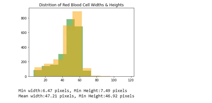

7. Splitting the Dataset into Training and Testing Sets

Splits the dataset into training and testing sets using scikit-learn's train_test_split function.

from sklearn.model_selection import train_test_split

testFraction = 0.2
trainSampleFilenames, testSampleFilenames = train_test_split(list(imgDict.keys()), test_size=testFraction, random_state=0xDEADBEEF)

8. Processing Images for Subregion Extraction

Creates a binary mask (bgMask) for the background using the annotated bounding boxes.

Calculates histograms of the hue channel for background regions.

Masks the original image with the background mask and flattens it for further processing.

Separates subregions corresponding to red blood cells (rbcSubImages) and white blood cells (wbcSubImages) based on the annotated labels.

import matplotlib.pyplot as plt

rbcSubImages = []
wbcSubImages = []
bgHistList = []

for trainFileName in trainSampleFilenames:
    hueOnly = imgDict[trainFileName][:,:,0]
    labels = imgLabelDict[trainFileName]
    bgMask = np.zeros(hueOnly.shape, np.uint8)
    bgMask.fill(255) #Initially all visible, will mask out cell regions later
    for label in labels:
        bgMask[label.top:label.bot,label.left:label.right] = 0#mask out fg (wbc or rbc)
        subImage = hueOnly[label.top:label.bot,label.left:label.right]
        if label.type == "rbc":
            rbcSubImages.append(subImage)
        else:
            wbcSubImages.append(subImage)
    bgHist = cv.calcHist([hueOnly], [0], bgMask, [181], [0, 181])
    bgHistList.append(bgHist[:,0])
            
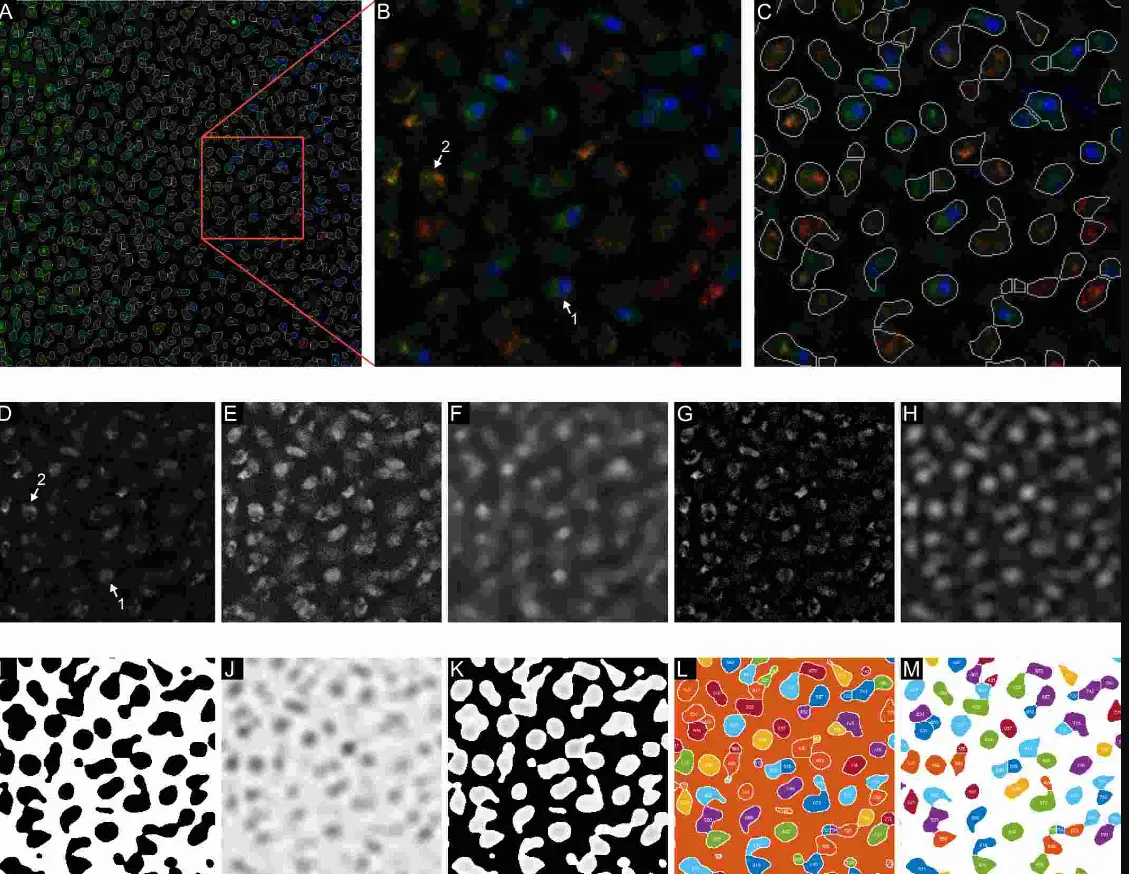
print("(Training Set) No. of rbc:{0}, wbc:{1}".format(len(rbcSubImages), len(wbcSubImages)))

The dataset is initially divided into training and test sets using an 80-20 split. Sub-images representing individual red blood cells, identified by their bounding boxes, are then extracted.

Simultaneously, the background—comprising the image regions not designated as either red blood cells or white blood cells—is also isolated.

To discern the dominant color characteristics of these two-pixel classes, the mean histogram is computed.

This analysis reveals a distinct correlation between the pixel hues and the respective classes; specifically, a greenish cyan hue is prevalent in the background, while a red hue characterizes the red blood cells.

Utilizing the statistical probability of each hue belonging to either the background or red blood cell class, a classification system is implemented for pixel categorization.

Notably, the class-prior probability term is omitted in the Naive Bayes Classifier (NBC) in this particular case.

This methodology enhances the understanding of the pixel distribution within the images and aids in the accurate classification of pixels based on their color characteristics.

9. Analyzing Histograms

Calculates histograms for red blood cells, white blood cells, and background from the extracted subregions.

Visualizes the histograms in a plot.

def normalizeHistogram(hist):
    return hist / np.sum(hist)

hsvGradient = cv.cvtColor(np.array([[[h, 255, 255] for h in np.arange(0, 181, dtype=np.uint8)]], dtype=np.uint8), cv.COLOR_HSV2RGB )

rbcPixelProb = normalizeHistogram(rbcHistogram)
wbcPixelProb = normalizeHistogram(wbcHistogram)
bgPixelProb = normalizeHistogram(bgHistogram)

plt.figure(figsize=(12,6))
plt.title("Fraction of each Hue(0-180) in each image category")
plt.imshow(hsvGradient, origin='lower',aspect='auto')
plt.gca().set_ylim(0,0.2)
plt.plot(rbcPixelProb, color="tab:red",linestyle="-", label="Red Blood Cell")
plt.plot(wbcPixelProb, color="white", linestyle="-.", label="White Blood Cell")
plt.plot(bgPixelProb, color="tab:cyan", label="Background")
plt.legend()

print("Peak hue for BG:{0}, WBC:{1}".format(np.argmax(bgPixelProb), np.argmax(rbcPixelProb)))

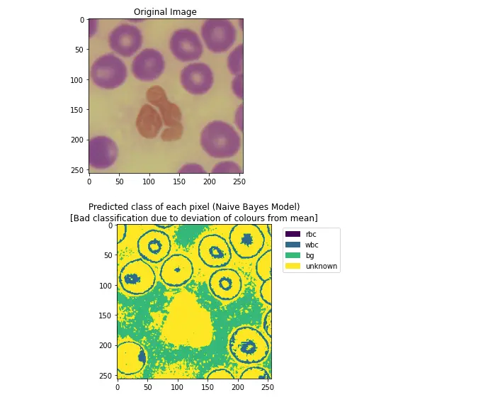
10. Chroma-Correction on source images

Simply applying the NBC classifier that was obtained using the mean color probabilities results in poor classification for some images (i.e. second pair shown below, where most of the image is simply marked as unknown).

Poor pixel classification occurs if the color distribution of an image varies too greatly from the mean of the image set.

Since each pixel class corresponds strongly to a single hue peak, color correction can be performed by roughly identifying the target color peak within an image and shifting it closer to the statistical mean.

import matplotlib.patches as mpatches

#hsvImage -> np.uint8[][]
def CrudePixelClassification(hsvImage):
    (height, width, _) = hsvImage.shape
    markedArray = np.zeros((height, width), dtype=np.uint8) 
    for row in range(height):
        for col in range(width):
            pixelHue = hsvImage[row,col,0]
            probabilities = [rbcPixelProb[pixelHue], wbcPixelProb[pixelHue], bgPixelProb[pixelHue]]
            maxVal = max(probabilities)
            noiseThreshold = 0.005
            markedArray[row,col] = probabilities.index(maxVal) if maxVal > noiseThreshold else len(probabilities)
    return markedArray
            
trainImgList = [imgDict[path] for path in trainSampleFilenames]

testImg = trainImgList[1]
markedPixels = CrudePixelClassification(testImg)

def PlotMarkedPixelGraph(markedPixels, hsvImg, optionalCaption=None):
    plt.title("Original Image")
    plt.imshow(cv.cvtColor(hsvImg, cv.cv2.COLOR_HSV2BGR))
    plt.show()
    
    hMarked = plt.imshow(markedPixels)
    additionalCaption = "\n" + optionalCaption if optionalCaption != None else ""
    plt.title("Predicted class of each pixel (Naive Bayes Model)" + additionalCaption)
    colors = [ hMarked.cmap(hMarked.norm(level)) for level in range(4)]
    patches = [ mpatches.Patch(color=colors[index], label=labelName) for index,labelName in enumerate(["rbc", "wbc", "bg", "unknown"])]
    plt.legend(handles=patches, bbox_to_anchor=(1.05, 1), loc=2)
    plt.show()
    
PlotMarkedPixelGraph(markedPixels, testImg)

skewedColorImg = trainImgList[2]
markedPixelsFailure = CrudePixelClassification(skewedColorImg)
PlotMarkedPixelGraph(markedPixelsFailure, skewedColorImg, "[Bad classification due to deviation of colours from mean]")

11. Color Correction based on Hue Distribution in an Image

The overall code performs color correction on an image based on the distribution of hue values.

Here's a step-by-step explanation:

Importing Libraries: Imported necessary libraries for Gaussian filtering (gaussian_filter1d) and peak detection (find_peaks).

HueDistance Function: Defined a function HueDistance to calculate the circular distance between two hue values in the range [0, 180].

GetHueHistogram Function: Defined a function GetHueHistogram that calculates the histogram of hue values in an input image in the HSV color space.

GetClosestPeak Function:  A function GetClosestPeak to find the index of the closest peak to a reference point in a set of peak indices, considering a maximum allowed distance.

GetHueCorrectionMap Function: Defines a function GetHueCorrectionMap that generates a hue correction map. This map is designed to adjust the actual hue values in the image to be closer to specified reference hue values.

ApplyColourCorrectionMap Function: Defines a function ApplyColourCorrectionMap that applies the generated hue correction map to the hue channel of an input HSV image.

Histogram Calculation and Smoothing:

Calculates the hue histogram of the input image (skewedColorImg).

Applies Gaussian smoothing to the histogram.

Peak Detection:

Sets expected background and RBC hues.

Detects peaks in the smoothed histogram using find_peaks.

Closest Peak Search:

Defines a search width (peakSearchWidth) for finding the closest peaks.

Finds the closest peaks to the expected background and RBC hues.

Hue Correction Map Generation:

Generates a hue correction map using the detected peaks and expected hues.

Applying Color Correction:

Applies the generated hue correction map to the input image (skewedColorImg) to obtain the final corrected image (correctedImage).

Printing Results:

Prints the detected RBC and background peaks.

from scipy.ndimage import gaussian_filter1d
from scipy.signal import find_peaks

def HueDistance(hue1, hue2):
    #for [0-180] hues
    diff = hue1 - hue2
    return ((diff + 90) % 180) - 90

def GetHueHistogram(hsvImage):
    return cv.calcHist([hsvImage], [0] , None, [181], [0, 181])[:,0]

def GetClosestPeak(huePeakIndices, referencePoint, maxDistance):
    if len(huePeakIndices) == 0:
        return referencePoint
    
    distances =  np.abs([HueDistance(hue, referencePoint) for hue in huePeakIndices])
    minIdx = np.argmin(distances)
    minDist = distances[minIdx]
    return huePeakIndices[minIdx] if minDist <= maxDistance else referencePoint

#Produces a hue map that converts the actual hue to a value that more closely matches the reference hue
def GetHueCorrectionMap(refBGHue, actualBgHue, refRBCHue, actualRBCHue, correctionWidth):
    def GetSingleHueCorrectionMap(refHue, actualHue):
        distFromActualPeak = np.abs([HueDistance(hue, actualHue) for hue in range(181)]) 
        bgCorrectionFactor = np.maximum((correctionWidth - distFromActualPeak) / correctionWidth, 0) #range from 0 - 1, 1 at the actualHue, 0 at a distance of correctionWidth from the actualHue (on both ends)
        actual2RefShift = refHue - actualHue #amount that needs to be added to the actual image to match the refence
        correctionMap = bgCorrectionFactor * actual2RefShift
        return correctionMap #Add this to the unity map to get a correction map 
    
    unityMapping = np.arange(181)
    bgCorrection = GetSingleHueCorrectionMap(refBGHue, actualBgHue)
    rbcCorrection = GetSingleHueCorrectionMap(refRBCHue, actualRBCHue)
   
    correctionMap = (unityMapping + bgCorrection + rbcCorrection)
    return np.abs(np.fmod(np.round(correctionMap), 181)).astype(np.uint8)

def ApplyColourCorrectionMap(hsvImage, colorCorrectionMap):
    paddedColorMap = np.zeros(256).astype(np.uint8)
    paddedColorMap[0:181] = colorCorrectionMap
    colorCorrected = np.copy(hsvImage)
    colorCorrected[:,:,0] = paddedColorMap[hsvImage[:,:,0]]    
    return colorCorrected


histogram = GetHueHistogram(skewedColorImg)
smoothedHistogram = gaussian_filter1d(histogram,5)

expectedBGHue = 71 
expectedRBCHue = 168 
peaksIndices, _ = find_peaks(smoothedHistogram, distance=10)

peakSearchWidth = 30
detectedRBCPeak = GetClosestPeak(peaksIndices, expectedRBCHue, peakSearchWidth)
detectedBGPeak = GetClosestPeak(peaksIndices, expectedBGHue, peakSearchWidth)
print(detectedRBCPeak, detectedBGPeak)

colorCorrectionMap = GetHueCorrectionMap(expectedBGHue, detectedBGPeak, expectedRBCHue, detectedRBCPeak, peakSearchWidth)
correctedImage = ApplyColourCorrectionMap(skewedColorImg, colorCorrectionMap)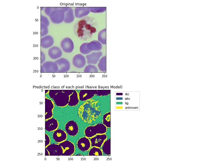

The code aims to correct the color balance of an image by adjusting the hue values based on the distribution of hues, with a focus on the background and RBC regions.

The correction is achieved through the generation of a hue correction map, which is then applied to the original image.

12. Chroma-Correction Strategy

Due to the rarity of White-Blood Cells, the histogram of each image typically only has two peaks (Red-RBCs and Green-Background).

Running peak detection on the smoothed histogram allows these peaks to be found.

Which can be shifted linearly to the expected mean hues of 71 (green background) & 168 (red-blood cells).

plt.figure(figsize=(12,6))
plt.title("Detected Hue Peaks")
plt.plot(histogram, "b", label="Raw Hue Distribution")
plt.plot(smoothedHistogram, "r--", label="Smoothed Hue Peaks")
plt.plot(peaksIndices, smoothedHistogram[peaksIndices], "x")
plt.xlabel("Hue")
plt.ylabel("No. of pixels")
plt.legend()
plt.show()

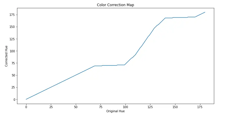
plt.figure(figsize=(12,6))
plt.title("Color Correction Map")
plt.xlabel("Original Hue")
plt.ylabel("Corrected Hue")
plt.plot(colorCorrectionMap)
plt.show()

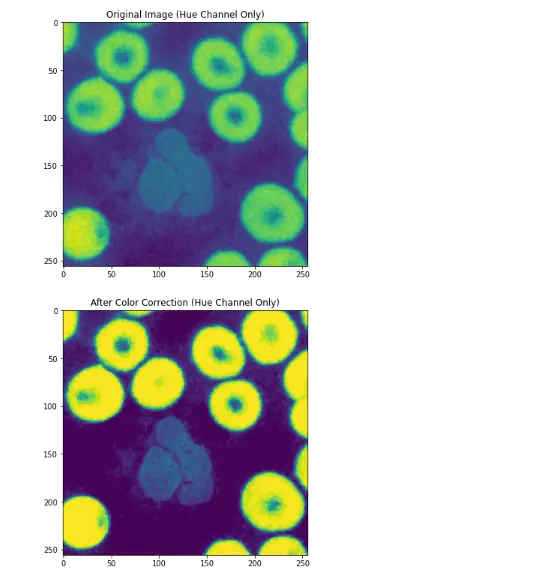
hueOnly = skewedColorImg[:,:,0]
plt.figure(figsize=(12,6))
plt.title("Original Image (Hue Channel Only)")
plt.imshow(hueOnly)
plt.show()

plt.figure(figsize=(12,6))
plt.title("After Color Correction (Hue Channel Only)")
plt.imshow(correctedImage[:,:,0])
plt.show()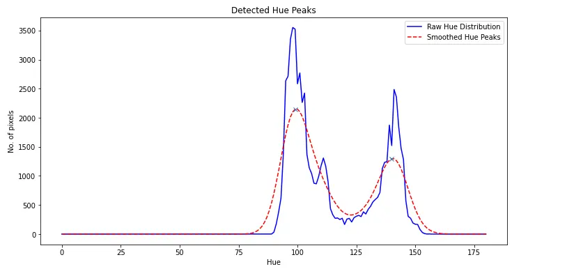

13. Pixel Classification using NBC

With the image-color variation issue settled, the NBC can then be applied to each color-corrected image to mark each pixel as potential red blood cells.

The translucency of the nuclei tends to result in a false negative within that region, resulting in "holes" present in the cell.

If these "holes" are unaddressed, applying the distance transform later will incorrectly generate too many local maxima around the holes, which results in over-segmentation of the cells.

def ApplyColorCorrectionToImage(hsvImage):
    histogram = GetHueHistogram(hsvImage)
    smoothedHistogram = gaussian_filter1d(histogram,5)
    
    expectedBGHue = 71 
    expectedRBCHue = 168 
    peaksIndices, _ = find_peaks(smoothedHistogram, distance=10)
    
    peakSearchWidth = 30
    detectedRBCPeak = GetClosestPeak(peaksIndices, expectedRBCHue, peakSearchWidth)
    detectedBGPeak = GetClosestPeak(peaksIndices, expectedBGHue, peakSearchWidth)
    
    colorCorrectionMap = GetHueCorrectionMap(expectedBGHue, detectedBGPeak, expectedRBCHue, detectedRBCPeak, peakSearchWidth)
    correctedImage = ApplyColourCorrectionMap(hsvImage, colorCorrectionMap)
    return correctedImage

colourCorrectedExample = ApplyColorCorrectionToImage(skewedColorImg)
ccMarkedPixels = CrudePixelClassification(colourCorrectedExample)
PlotMarkedPixelGraph(ccMarkedPixels, colourCorrectedExample)

14. Filling of Small holes caused by poor Nuclei classification  and Distance Transform

Since this classification problem only involves 2 classes (non RBC & RBC), the 3 non-RBC classes (White-Blood Cells, Background & Unknown) are lumped together into a single non-RBC class.

A median filter is first run on this new mask to remove noise.

Holes are identified as regions of connected non-RBC pixels that are under a specified height & width.

These are removed by flood-filling them with the markers for RBCs.

The distance transform is then taken to identify the "innermost" pixels within each region.

These innermost regions are taken as the starting points (basins) for the watershed algorithm.

from skimage.feature import peak_local_max
import math

def FilterOutLabel(inputImage, targetLabel):
    return np.equal(inputImage,targetLabel).astype(np.uint8)

def MedianFilter(inputImage):
    medBlurred = cv.medianBlur(inputImage, 7) 
    #kernel = cv.getStructuringElement(cv.MORPH_ELLIPSE, (7,7))
    #return  cv.morphologyEx(medBlurred, cv.MORPH_CLOSE, kernel, iterations=2)
    return medBlurred

def DistanceMapToNonRBCLabel(inputImage):
    return cv.distanceTransform(inputImage,cv.DIST_L2,3)

def DrawMarkerSeeds(cellMask, cellLabelWithinMask, markerList):
    markerBuffer = np.zeros(distanceTransform.shape, dtype=np.int32)
    for idx,coord in enumerate(markerList):
        (height,width) = cellMask.shape
        (maxRow, maxCol) = (height-1, width - 1)
        [row,col] = coord
        radius = 7 #cv.watershed seems to merge clusters together if the region seed is too small
        markerIdx = idx + 2 #0 reserved for indeterminate regions, 1 reserved for BG
        markerBuffer[max(row-radius,0):min(row+radius,maxRow),max(col-radius,0):min(col+radius,maxCol)] = markerIdx
        
    markerBuffer[cellMask==cellLabelWithinMask] = 1 #Give BG its own marker
    return markerBuffer

# 1 = perfectly spherical, numbers closer to 0 = less spherical
def Sphericity(width, height, area):
    diameter = max(width,height)
    expectedArea = 0.25 * math.pi * (diameter ** 2)
    sphericity = 1 - abs(expectedArea - area) / expectedArea
    return sphericity

def FillHolesInMask(maskImg, maxHoleSize, fillLabel):
    (_,labels,statList, _) = cv.connectedComponentsWithStats(np.max(maskImg)-maskImg, connectivity=8) 
    filledBuffer = np.copy(maskImg)
    for label,stats in enumerate(statList):
        (x,y,width,height,area) = stats
        isNuclei = Sphericity(width, height, area) > 0.3
        if (width <= maxHoleSize) and (height <= maxHoleSize) and isNuclei:
            filledBuffer[labels==label] = fillLabel
    return filledBuffer
    
rbcLabelsOnly = FilterOutLabel(markedPixels, 0)
plt.title("RBC and non-RBC mask")
plt.imshow(rbcLabelsOnly)
plt.show()

rbcSmoothed = MedianFilter(rbcLabelsOnly)
plt.title("Mask after de-noising\n(Median Filter)")
plt.imshow(rbcSmoothed)
plt.show()

rbcHolesRemoved = FillHolesInMask(rbcSmoothed, 40, 1)
plt.title("Mask after hole-removal")
plt.imshow(rbcHolesRemoved)
plt.show()

distanceTransform = DistanceMapToNonRBCLabel(rbcHolesRemoved)
localMaximaCoordinates = peak_local_max(distanceTransform,exclude_border=False, min_distance=22)
plt.title("Distance Transform\n(Maxima marked in red)")
plt.imshow(distanceTransform)
plt.plot(localMaximaCoordinates[:,1], localMaximaCoordinates[:,0], 'r.')
plt.show()

markers = DrawMarkerSeeds(rbcHolesRemoved, 0, localMaximaCoordinates)

plt.title("Markers\n(Each color represents one starting point for segmentation)")
plt.imshow(markers)
plt.show()

_3ChannelGrayscale = cv.cvtColor(255 - rbcHolesRemoved*255, cv.COLOR_GRAY2BGR).astype(np.uint8)
plt.title("Watershed Heightmap\n(White is basically impassable)")
plt.imshow(_3ChannelGrayscale)
plt.show()


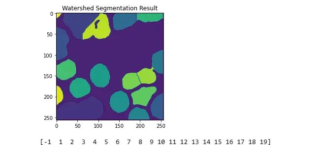
segmented = cv.watershed(_3ChannelGrayscale, markers)
plt.title("Watershed Segmentation Result")
plt.imshow(segmented)
plt.show()
print(np.unique(segmented))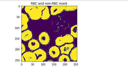

15. Image Segmentation and Cell Bounding Boxes

The code focuses on segmenting cells in an image based on its HSV color representation using the watershed algorithm.

Additionally, it extracts bounding boxes around the segmented cells and visualizes the results.

Here's an overall explanation:

15.1 Image Segmentation using Watershed Algorithm

The SegmentImage function takes an HSV image as input and performs the following steps:

Pixel Classification: Classifies pixels using the CrudePixelClassification function.

Filtering and Denoising: Filters out the background using the FilterOutLabel function and applies median filtering with MedianFilter.

Hole Removal: Removes holes in the mask using FillHolesInMask.

Distance Transform: Computes a distance map to a non-RBC (Red Blood Cell) label using DistanceMapToNonRBCLabel.

Local Maxima Detection: Identifies local maxima in the distance map using peak_local_max.

Marker Seeds Generation: Generates marker seeds for watershed segmentation with DrawMarkerSeeds.

Watershed Segmentation: Applies the watershed algorithm using OpenCV's cv.watershed.

15.2 Bounding Box Extraction:

The GetCellBoundingBoxes function extracts bounding boxes around the segmented cells. It iterates through unique labels in the segmented image and creates bounding boxes for each cell.

15.3 Visualization:

The PlotSegmentedImageAndBoundingBoxes function generates a visual comparison of the original HSV image and the segmented cells.

It uses Matplotlib to create a side-by-side subplot with the original image, bounding boxes, and the segmented image with corresponding bounding boxes drawn in red.

15.4 Test and Visualization:

Finally, the code selects a test image from a list (trainImgList), performs segmentation using the SegmentImage function, extracts bounding boxes using GetCellBoundingBoxes, and visualizes the results using PlotSegmentedImageAndBoundingBoxes.

from matplotlib.patches import Rectangle

#(hsvImage:HSV image) => (segmentedImage:int32[][]  - -1 for watershed boundaries, 1 for bg, +ve integers represent label for connected components) 
def SegmentImage(hsvImage):
    classifiedPixels = CrudePixelClassification(hsvImage)
    rbcOnly = FilterOutLabel(classifiedPixels, 0)
    rbcDenoised = MedianFilter(rbcOnly)
    rbcHolesRemoved = FillHolesInMask(rbcDenoised, 40, 1)
    distanceTransform = DistanceMapToNonRBCLabel(rbcHolesRemoved)
    
    localMaximaCoordinates = peak_local_max(distanceTransform,exclude_border=False, min_distance=10)
    markerSeeds = DrawMarkerSeeds(rbcHolesRemoved, 0, localMaximaCoordinates)
    
    bgrGrayscaleHeightMap =  cv.cvtColor(255 - rbcHolesRemoved*255, cv.COLOR_GRAY2BGR).astype(np.uint8)
    segmentedCells = cv.watershed(bgrGrayscaleHeightMap, markerSeeds)
    return segmentedCells 

#type = ['rbc'|'wbc']
#CellLabel = namedtuple('CellLabel', ['left', 'top', 'right', 'bot', 'type'])

def GetCellBoundingBoxes(segmentedImage):
    allLabels = np.unique(segmentedImage)
    cellLabels = allLabels[allLabels > 1]
    boundingBoxList = []
    for cellLabel in cellLabels:
        cellMask = np.equal(segmentedImage, cellLabel).astype(np.uint8) #inefficient, but probably still faster than a BFS in python
        rect = cv.boundingRect(cellMask)
        boundingBoxList.append(CellLabel(rect[0], rect[1], rect[0] + rect[2], rect[1] + rect[3], "rbc"))
    return boundingBoxList

def PlotSegmentedImageAndBoundingBoxes(segmentedImg, boundingBoxList, hsvImage):
    fig, (ax1, ax2) = plt.subplots(1, 2)
    ax1.imshow(cv.cvtColor(hsvImage, cv.COLOR_HSV2RGB))
    ax1.set_title("Original Picture &\nBounding Boxes")
    ax2.imshow(segmentedImg)
    ax2.set_title("Segmented Cells &\nBounding Boxes")
    for boundingBox in boundingBoxList:
        (width, height) = (boundingBox.right - boundingBox.left, boundingBox.bot - boundingBox.top)
        ax1.add_patch(Rectangle((boundingBox.left, boundingBox.top), width, height, color="red",fill=None))
        ax2.add_patch(Rectangle((boundingBox.left, boundingBox.top), width, height, color="red",fill=None))
    plt.show()
        
testImg = trainImgList[6]         
segmentedImg = SegmentImage(testImg)
boundingBoxes = GetCellBoundingBoxes(segmentedImg)
PlotSegmentedImageAndBoundingBoxes(segmentedImg, boundingBoxes, testImg)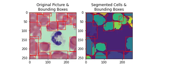

The code provides a comprehensive pipeline for segmenting cells in an image, extracting bounding boxes, and visually assessing the segmentation results.

The watershed algorithm, along with other image processing techniques, plays a crucial role in achieving accurate cell segmentation.

16. Parallel Image Segmentation with Multiprocessing

This code snippet appears to be using the multiprocessing module in Python to parallelize the processing of a list of images (trainImgList).

The main goal seems to be performing image segmentation on each image in parallel using multiple processes.

Here's a breakdown of the code:

Import the Pool class from the multiprocessing module.

Print the length of the trainImgList list.

Define a function ProcSegment that takes an HSV image as input, applies color correction using a function ApplyColorCorrectionToImage, performs image segmentation using a function SegmentImage, and then retrieves bounding boxes using a function GetCellBoundingBoxes.

The result is a tuple containing the segmented image and a list of bounding boxes.

Initialize an empty list cellSegmentations to store the results of the image segmentation process.

Use the Pool class to create a pool of worker processes. The number of processes in the pool is determined by the available system resources.

Use the map function of the Pool class to apply the ProcSegment function to each element in the trainImgList in parallel. This means that different images will be processed simultaneously by different processes.

The results (tuples of segmented images and bounding boxes) are collected in the cellSegmentations list.

from multiprocessing import Pool

print(len(trainImgList))

def ProcSegment(hsvImage):
    colorCorrected = ApplyColorCorrectionToImage(hsvImage)
    segmented = SegmentImage(colorCorrected)
    boundingBoxes = GetCellBoundingBoxes(segmented)
    return (segmented, boundingBoxes)

#(segmentationMap:int32[][], boundingBoxes:CellLabels[])[]
cellSegmentations = []

with Pool() as processPool:
    cellSegmentations = processPool.map(ProcSegment, trainImgList)

The code parallelizes the image segmentation process using the multiprocessing module, which can lead to significant speedup when processing a large number of images.

Each image is processed independently by a separate process in the pool, and the results are collected into a list for further analysis or storage.

for cellSegmentationData,hsvImg in list(zip(cellSegmentations,trainImgList))[0:5]:
    (segmentation, boundingBoxes) = cellSegmentationData
    PlotSegmentedImageAndBoundingBoxes(segmentation, boundingBoxes, hsvImg)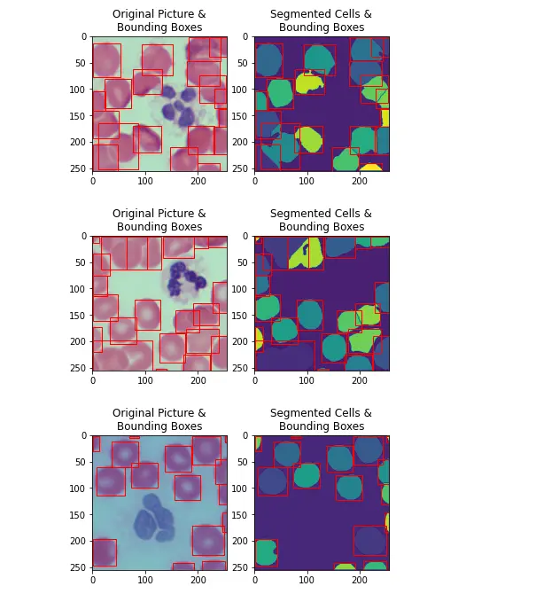

17. Evaluation Metrics

Intersection-Over-Union is a simple metric that describes how closely two regions overlap.

It is the ratio of the area of the overlapping regions and the combined area of of the regions. An IOU of 1 represents a perfect match, whilst an IOU of 0 represents no overlap at all.

Due to the denominator being the combined area of both regions, this metric also penalizes predictions that are excessively large in comparison to the ground truth.

Due to the nature of the Watershed Algorithm, the number of predicted Red-blood cells may not match with the ground truth.

As such, deciding which predictions & ground truth pairs to calculate the IOU with becomes an open question.

For this notebook, ground-truth bounding boxes are matched with the prediction whose centre is the closest.

Once paired, each ground truth / prediction will not be used in another IOU calculation.

To achieve the global optimal pairing of ground-truths & predictions based on their distances, a min-weight bipartitate match is deployed.

Bounding boxes with no available match are simply ignored.

from scipy.sparse import csr_matrix
from scipy.sparse.csgraph import min_weight_full_bipartite_matching

def CellLabelCentre(cellLabel):
    xCentre = 0.5 * (cellLabel.right + cellLabel.left)
    yCentre = 0.5 * (cellLabel.top + cellLabel.bot)
    return (xCentre, yCentre)

def EuclideanDist(coord1, coord2):
    return math.hypot(coord1[0] - coord2[0], (coord1[1] - coord2[1]))

def GetCellBoundingBoxArea(cellLabel):
    width = cellLabel.right -  cellLabel.left
    height = cellLabel.bot - cellLabel.top 
    return width * height

def GetIOU(cellLabel1, cellLabel2):
    def SafeDiv(numerator, denominator):
        if numerator == 0 and denominator == 0:
            return 0
        elif denominator == 0:
            return sys.float_info.max
        else:
            return numerator / denominator
    
    def Overlap(min1, max1, min2, max2):
        return max(0, min(max1, max2) - max(min1, min2))
    
    xIntersection = Overlap(cellLabel1.left, cellLabel1.right, cellLabel2.left, cellLabel2.right)
    yIntersection = Overlap(cellLabel1.top, cellLabel1.bot, cellLabel2.top, cellLabel2.bot)
    
    intersectionArea = xIntersection * yIntersection
    unionArea = GetCellBoundingBoxArea(cellLabel1) +  GetCellBoundingBoxArea(cellLabel2) - intersectionArea
    
    #IOU ranges from 0-1
    return max(SafeDiv(intersectionArea, unionArea), 0)
    

#CellLabel = namedtuple('CellLabel', ['left', 'top', 'right', 'bot', 'type'])
def GetIOUScore(groundTruth, predictions):
    groundTruthCentres = [CellLabelCentre(label) for label in groundTruth]
    predictionCentres = [CellLabelCentre(label) for label in predictions]
    #groundTruth -> prediction
    #adjGraph[groundTruthIdx][predictedIndex] -> distance
    adjGraph = []
    for srcPoint in groundTruthCentres:
        #add one to cater to the min-weight bipartite matching algorithm
        distances = [EuclideanDist(srcPoint, destPoint) + 1 for destPoint in predictionCentres]
        adjGraph.append(distances)
    biadjacency_matrix = csr_matrix(adjGraph)
    groundTruth_ind, prediction_ind = min_weight_full_bipartite_matching(biadjacency_matrix)
    
    matchedGroundTruthLabels = [groundTruth[index] for index in groundTruth_ind]
    matchedPredictedLabels = [predictions[index] for index in prediction_ind]
    
    iouScoreList = []
    
    for actual, predicted in zip(matchedGroundTruthLabels, matchedPredictedLabels):
        iou = GetIOU(actual, predicted)
        iouScoreList.append((iou, actual, predicted))
    
    #no penalty applied for false positives / unidentified cells
    meanIOU = (
        np.mean([iou for iou,_,_ in iouScoreList]) 
        if len(iouScoreList) > 0 
        else 0)
    
    return (meanIOU, iouScoreList)

#list for each image
trainCellLabelsList = [imgLabelDict[filename] for filename in trainSampleFilenames]
predictedTrainCellLabelsList = [cellLabel for _, cellLabel in cellSegmentations]

imgMeanAndMatches = []
for imgLabel, imgPredictions in zip(trainCellLabelsList, predictedTrainCellLabelsList):
    mean, matchedPredictionList = GetIOUScore(imgLabel, imgPredictions)
    imgMeanAndMatches.append((mean, matchedPredictionList))

means = [mean for mean, _ in imgMeanAndMatches]
print("Mean of mean IOUs:{:.2f}%".format(np.mean(means) * 100))

18. Segmentation results on Test Image set

testImgList = [imgDict[path] for path in testSampleFilenames]

testSetSegmentations = []

with Pool() as processPool:
    testSetSegmentations = processPool.map(ProcSegment, testImgList)
    
for cellSegmentationData,hsvImg in list(zip(testSetSegmentations,testImgList)):
    (segmentation, boundingBoxes) = cellSegmentationData
    PlotSegmentedImageAndBoundingBoxes(segmentation, boundingBoxes, hsvImg)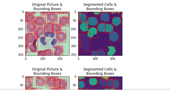

19. Test Image Set IOU results

The IOUs produced by the watershed approach follow a bimodal distribution. A significant fraction (13%) fail to create any significant overlap with the ground truth (< 0.2 IOU score) and can simply be interpreted as misidentified Red-Blood Cells.

The second peak in the Bimodal distribution (>= 0.2 IOU) has a mean of 0.72, and can be construed as the accuracy when running Watershed Segmentation on correctly identified RBC regions.

Given that misclassification of regions as RBC appears to be an issue, more sophisticated methods to perform the preliminary pixel classification could be used (i.e. Grabcut to iterately refine the red-blood cell regions) if higher accuracy is required.

#list for each image
testCellLabelsList = [imgLabelDict[filename] for filename in testSampleFilenames]
predictedTestCellLabelsList = [cellLabel for _, cellLabel in testSetSegmentations]

matchedIOUs = []

for imgLabel, imgPredictions in zip(testCellLabelsList, predictedTestCellLabelsList):
    mean, matchedPredictionList = GetIOUScore(imgLabel, imgPredictions)
    iousOnly =  [iou for (iou,_,_) in matchedPredictionList]
    matchedIOUs.extend(iousOnly) 

nMatchedLabels = len(matchedIOUs)
nGroundTruthLabels = np.sum([len(labelList) for labelList in testCellLabelsList])
nPredictedLabels = np.sum([len(labelList) for labelList in predictedTestCellLabelsList])


print("Mean IOU for matched bounding boxes {:.2f}%".format(np.mean(matchedIOUs) * 100))
print("No. of ground truth bounding boxes: {0},\nNo. of predicted bounding boxes: {1}\nNo. of matched bounding boxes: {2}".format(nGroundTruthLabels, nPredictedLabels, nMatchedLabels))

print("---")
node1 = [iou for iou in matchedIOUs if iou < 0.2]
node2 = [iou for iou in matchedIOUs if iou >= 0.2]
print("Size of node1:{}, mean={:.2f}\nSize of node2:{}, mean={:.2f}, median={:.2f}".format(len(node1), np.mean(node1), len(node2), np.mean(node2), np.median(node2)))

plt.figure(figsize=(12,6))
plt.title("Distribution of Intersection Over Union Scores")
plt.ylabel("No. of bounding boxes")
plt.xlabel("IOU Score (0 to 1)")
plt.hist(matchedIOUs)
plt.show()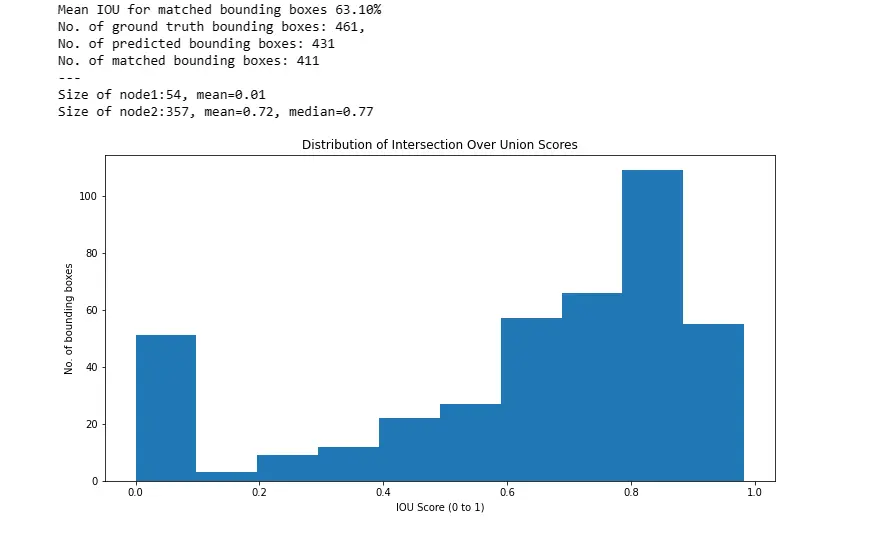

Conclusion

This hands-on tutorial demonstrates the robust application of the Watershed Algorithm in cell segmentation, particularly focusing on red blood cells—a critical aspect in biotechnology and life sciences.

The methodology, integrating machine learning, color correction strategies, and parallel processing, offers a holistic approach for researchers and practitioners.

By addressing challenges such as pixel misclassification and optimizing for accurate segmentation, this blog empowers machine learning experts, researchers, product managers, and bio-technologists to advance their capabilities in image analysis.

The bimodal distribution of Intersection-Over-Union results provides insights into the algorithm's performance, guiding future refinements for even higher accuracy.

As we navigate the intersection of technology and life sciences, this tutorial serves as a valuable resource, fostering innovation and progress in the dynamic field of cell segmentation.

Frequently Asked Questions

1. Why is watershed based cell segmentation under-segmentation?

Watershed-based cell segmentation can suffer from under-segmentation due to the algorithm's tendency to merge adjacent regions that share similar intensity or color characteristics.

This occurs when the algorithm interprets nearby cells as part of the same region, resulting in the under-segmentation of individual cells.

2. What is a watershed algorithm?

The watershed algorithm is a digital image processing technique used for segmentation and object recognition.

It treats pixel intensities as elevation values and simulates a flooding process.

Watershed lines represent boundaries between regions, separating areas with different pixel characteristics.

The algorithm is commonly applied in image segmentation to identify and separate distinct objects or regions within an image.

3. Can SM-watershed cell segmentation be used to identify missing cells?

Yes, SM-watershed cell segmentation can be utilized to identify missing cells.

The watershed algorithm, particularly in the context of cell segmentation, analyzes image regions based on intensity or color differences.

By examining the segmented regions, discrepancies or gaps in the expected cell pattern can be detected, enabling the identification of missing cells within the image.

Looking for high quality training data to train your cell segmentation model? Talk to our team to get a tool demo.