ML Begineer's Guide on Network Intrusion Detection

Introduction

This is a comprehensive guide on Network Intrusion Detection Systems (NIDS).

The blog is tailored for both beginners and experts in machine learning, product managers, and researchers interested in building effective intrusion detection systems.

Network Intrusion Detection is vital for identifying and responding to security threats within a network.

In this guide, we cover the entire process of building a robust system, from initial setup and data exploration to model implementation and performance evaluation.

Our hands-on tutorials showcase the use of various machine learning models, including traditional classifiers like KNN, Logistic Regression, and Decision Trees, as well as advanced techniques such as Random Forest, Gradient Boosting, and NLP concepts.

We highlight the relevance of NLP in enhancing textual data analysis for improved threat detection.

Whether you're a beginner starting your machine learning journey or an expert looking to enhance security measures, this guide provides valuable insights and practical guidance.

Dive in, explore, and empower yourself to contribute to the evolving landscape of cybersecurity.

Hands-On Tutorial

1. Import Packages and Configurations

The code begins by installing necessary Python packages, such as NumPy, Pandas, Seaborn, Matplotlib, Optuna, Scikit-learn, XGBoost, CatBoost, LightGBM, and other libraries.

Following the installations, it imports these packages and sets up configurations for the environment.

The code suppresses installation output and warning messages. It also configures Optuna's logging verbosity.

Subsequently, it imports various machine learning models and tools, including decision trees, k-nearest neighbors, logistic regression, support vector machines, ensemble methods (Random Forest, AdaBoost, Gradient Boosting), Naive Bayes, LightGBM, and XGBoost classifiers.

Additionally, it imports modules for data preprocessing, feature selection, and visualization.

Lastly, the code walks through the Kaggle input directory, printing the path of each file.

Overall, this script is a setup for a machine learning project, including essential library installations, configurations, and the importation of relevant tools for data analysis and modeling.

%pip install numpy pandas seaborn matplotlib optuna sklearn xgboost catboost lightgbm > /dev/null 2>&1

import numpy as np
import pandas as pd
import seaborn as sns
import matplotlib.pyplot as plt
from pandas.api.types import is_numeric_dtype
import warnings
import optuna
from sklearn import tree
from sklearn.model_selection import train_test_split
from sklearn.neighbors import KNeighborsClassifier
from sklearn.linear_model import LogisticRegression
from sklearn.preprocessing import StandardScaler, LabelEncoder
from sklearn.tree  import DecisionTreeClassifier
from sklearn.ensemble import RandomForestClassifier, AdaBoostClassifier, VotingClassifier, GradientBoostingClassifier
from sklearn.svm import SVC, LinearSVC
from sklearn.naive_bayes import BernoulliNB
from lightgbm import LGBMClassifier
from sklearn.feature_selection import RFE
import itertools
from catboost import CatBoostClassifier
from xgboost import XGBClassifier
from tabulate import tabulate
import os
warnings.filterwarnings('ignore')
optuna.logging.set_verbosity(optuna.logging.WARNING)
for dirname, _, filenames in os.walk('/kaggle/input'):
    for filename in filenames:
        print(os.path.join(dirname, filename))

2. Data Preprocessing and EDA

This code uses the Pandas library to read two CSV files, 'Train_data.csv' and 'Test_data.csv', located in the Kaggle input directory.

The data from these files is loaded into two Pandas DataFrames, namely 'train' and 'test'.

The 'train' DataFrame contains the training data, which is presumably used to train machine learning models, while the 'test' DataFrame holds the test data for evaluating the model's performance.

The last line, 'train', is used to display the contents of the 'train' DataFrame, providing a glimpse of the dataset's structure and values.

This is a common initial step in a machine learning project where data is loaded and inspected to better understand its characteristics before proceeding with analysis and modeling.

train=pd.read_csv('/kaggle/input/network-intrusion-detection/Train_data.csv')
test=pd.read_csv('/kaggle/input/network-intrusion-detection/Test_data.csv')
train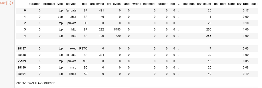

train.info()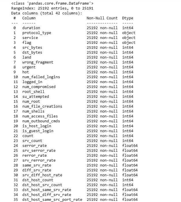

train.head()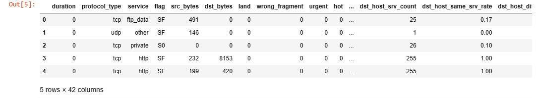

train.describe()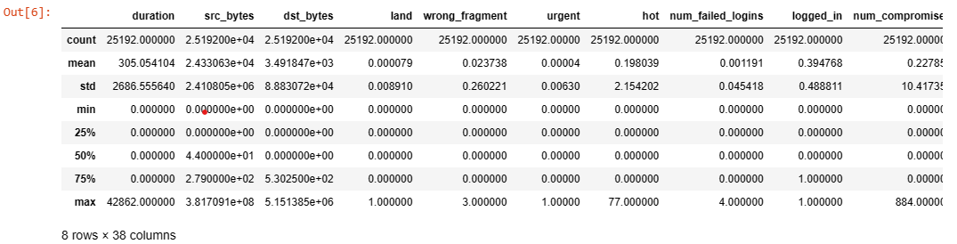

train.describe(include='object')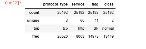

3. Handling Missing Data and Duplicates

The code calculates and prints the percentage of missing values for each column in the 'train' DataFrame.

It starts by obtaining the total number of rows in the DataFrame. Then, it identifies columns with missing values by checking if the sum of null values for a column is greater than zero.

For each such column, the code calculates the count and percentage of missing values and prints the result, indicating the column name, the count of missing values, and the percentage of missing values relative to the total number of rows.

This provides a quick overview of the missing data distribution in the training dataset, aiding in the decision-making process for handling missing values during the data preprocessing stage of a machine learning project.

total = train.shape[0]
missing_columns = [col for col in train.columns if train[col].isnull().sum() > 0]
for col in missing_columns:
    null_count = train[col].isnull().sum()
    per = (null_count/total) * 100
    print(f"{col}: {null_count} ({round(per, 3)}%)")

print(f"Number of duplicate rows: {train.duplicated().sum()}")

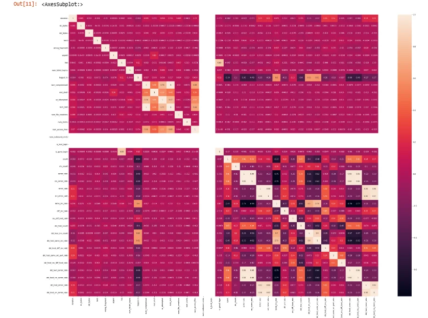
4. Visualizing and Plotting Graphs

plt.figure(figsize=(40,30))
sns.heatmap(train.corr(), annot=True)

sns.countplot(x=train['class'])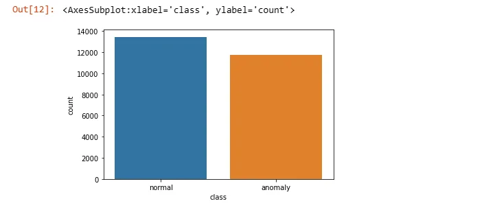

5. Label Encoding

The code defines a label encoding function, 'le', that takes a DataFrame 'df' as input and applies label encoding to transform categorical columns with 'object' data type into numerical representations using the LabelEncoder from scikit-learn.

The function iterates through each column in the DataFrame, checks if its data type is 'object', and if so, applies label encoding.

It is then used to encode both the 'train' and 'test' DataFrames.

Additionally, the code drops the column 'num_outbound_cmds' from both 'train' and 'test' DataFrames, likely due to its limited variability or redundancy.

Finally, the 'head()' method is used to display the first few rows of the modified 'train' DataFrame, showcasing the numerical representation of the categorical variables after label encoding.

This preprocessing step is common in machine learning to convert categorical features into a format suitable for training models that require numerical input.

def le(df):
    for col in df.columns:
        if df[col].dtype == 'object':
                label_encoder = LabelEncoder()
                df[col] = label_encoder.fit_transform(df[col])

le(train)
le(test)

train.drop(['num_outbound_cmds'], axis=1, inplace=True)
test.drop(['num_outbound_cmds'], axis=1, inplace=True)
train.head()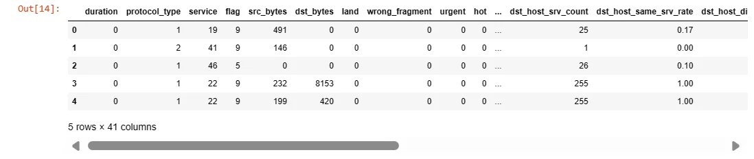

6. Feature selection

This part performs feature selection using the Recursive Feature Elimination (RFE) technique with a RandomForestClassifier.

It starts by separating the target variable 'class' from the features in the 'train' DataFrame, creating 'X_train' and 'Y_train'.

Then, it initializes a RandomForestClassifier and applies RFE with the goal of selecting the top 10 features.

The code creates a mapping of feature selection results, where each feature is paired with a boolean indicating whether it was selected or not.

Finally, it extracts the names of the selected features based on the RFE results.

This process helps identify a subset of features deemed most relevant for predicting the target variable, potentially improving model efficiency and interpretability by focusing on the most informative features.

X_train = train.drop(['class'], axis=1)
Y_train = train['class']

rfc = RandomForestClassifier()

rfe = RFE(rfc, n_features_to_select=10)
rfe = rfe.fit(X_train, Y_train)

feature_map = [(i, v) for i, v in itertools.zip_longest(rfe.get_support(), X_train.columns)]
selected_features = [v for i, v in feature_map if i==True]

selected_features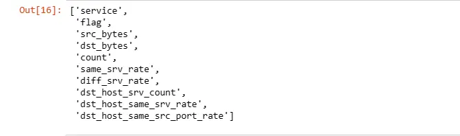

X_train = X_train[selected_features]

7. Splitting and Scaling data

This part involves the preprocessing steps of feature scaling and data splitting for a machine learning model.

It uses StandardScaler from scikit-learn to standardize the features in the training dataset, ensuring that they have a mean of 0 and a standard deviation of 1.

The scaled data is then used to replace the original feature values.

Additionally, the code employs the 'train_test_split' function to divide the training dataset into training and testing sets with a 70-30 split ratio.

This split facilitates model training on a subset of the data and subsequent evaluation on the unseen data.

Standardization is crucial for algorithms sensitive to the scale of input features, and splitting the data allows for assessing the model's generalization performance.

scale = StandardScaler()
X_train = scale.fit_transform(X_train)
test = scale.fit_transform(test)

x_train, x_test, y_train, y_test = train_test_split(X_train, Y_train, train_size=0.70, random_state=2)

8. K Nearest Neighbors (KNN) classification model

This code utilizes Optuna, a hyperparameter optimization library, to find the optimal number of neighbors for the K Nearest Neighbors (KNN) classification model.

The objective function defines a trial with a search space for the number of neighbors, and the study aims to maximize the classification accuracy on the test set.

After the optimization process, the best trial's parameters are retrieved, and a KNN model is trained with the optimal number of neighbors.

The code then evaluates and prints the training and testing accuracy scores of the KNN model on the provided dataset.

In this specific case, the optimal number of neighbors found is 15, and the resulting KNN model achieves high accuracy on both the training and testing sets, with a training score of approximately 97.7% and a testing score of approximately 97.7%.

def objective(trial):
    n_neighbors = trial.suggest_int('KNN_n_neighbors', 2, 16, log=False)
    classifier_obj = KNeighborsClassifier(n_neighbors=n_neighbors)
    classifier_obj.fit(x_train, y_train)
    accuracy = classifier_obj.score(x_test, y_test)
    return accuracy

study_KNN = optuna.create_study(direction='maximize')
study_KNN.optimize(objective, n_trials=1)
print(study_KNN.best_trial)

KNN_model = KNeighborsClassifier(n_neighbors=study_KNN.best_trial.params['KNN_n_neighbors'])
KNN_model.fit(x_train, y_train)

KNN_train, KNN_test = KNN_model.score(x_train, y_train), KNN_model.score(x_test, y_test)

print(f"Train Score: {KNN_train}")
print(f"Test Score: {KNN_test}")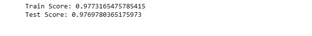

9. Logistic Regression Model

lg_model = LogisticRegression(random_state = 42)
lg_model.fit(x_train, y_train)

lg_train, lg_test = lg_model.score(x_train , y_train), lg_model.score(x_test , y_test)

print(f"Training Score: {lg_train}")
print(f"Test Score: {lg_test}")

10. Decision Tree Classifier

This part again employs Optuna for hyperparameter optimization to determine the optimal configuration for a Decision Tree Classifier.

The objective function defines a search space for the maximum depth and maximum features of the decision tree, with the goal of maximizing accuracy on the test set.

After optimizing over 30 trials, the best trial's parameters are retrieved, and a Decision Tree model is trained and evaluated on the provided dataset.

The results indicate a perfect training score of 100% accuracy and an impressive testing score of approximately 99.5%.

Additionally, the code generates a visualization of the trained decision tree using the plot_tree function from scikit-learn.

Furthermore, a bar plot is created to visualize the feature importance, showing the top features contributing to the decision tree's classification performance.

This analysis provides insights into the key features influencing the model's decisions.

def objective(trial):
    dt_max_depth = trial.suggest_int('dt_max_depth', 2, 32, log=False)
    dt_max_features = trial.suggest_int('dt_max_features', 2, 10, log=False)
    classifier_obj = DecisionTreeClassifier(max_features = dt_max_features, max_depth = dt_max_depth)
    classifier_obj.fit(x_train, y_train)
    accuracy = classifier_obj.score(x_test, y_test)
    return accuracy

study_dt = optuna.create_study(direction='maximize')
study_dt.optimize(objective, n_trials=30)
print(study_dt.best_trial)

dt = DecisionTreeClassifier(max_features = study_dt.best_trial.params['dt_max_features'], max_depth = study_dt.best_trial.params['dt_max_depth'])
dt.fit(x_train, y_train)

dt_train, dt_test = dt.score(x_train, y_train), dt.score(x_test, y_test)

print(f"Train Score: {dt_train}")
print(f"Test Score: {dt_test}")

fig = plt.figure(figsize = (30,12))
tree.plot_tree(dt, filled=True);
plt.show()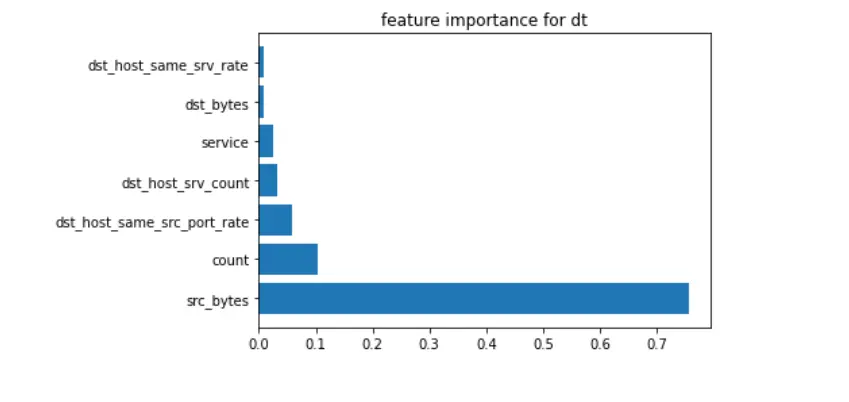

from matplotlib import pyplot as plt

def f_importance(coef, names, top=-1):
    imp = coef
    imp, names = zip(*sorted(list(zip(imp, names))))

    # Show all features
    if top == -1:
        top = len(names)

    plt.barh(range(top), imp[::-1][0:top], align='center')
    plt.yticks(range(top), names[::-1][0:top])
    plt.title('feature importance for dt')
    plt.show()

# whatever your features are called
features_names = selected_features

# Specify your top n features you want to visualize.
# You can also discard the abs() function 
# if you are interested in negative contribution of features
f_importance(abs(dt.feature_importances_), features_names, top=7)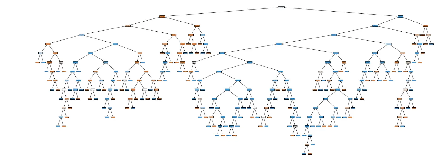

11. Random Forest Classifier

This code utilizes Optuna for hyperparameter optimization to determine the optimal configuration for a Random Forest Classifier.

The objective function defines a search space for the maximum depth, maximum features, and the number of estimators (trees) in the random forest, aiming to maximize accuracy on the test set.

After optimizing over 30 trials, the best trial's parameters are retrieved, and a Random Forest model is trained and evaluated on the provided dataset.

The results show high performance, with a near-perfect training score of approximately 99.9% accuracy and an impressive testing score of approximately 99.6%.

The code also generates a bar plot visualizing the feature's importance, providing insights into the key features contributing to the Random Forest model's classification decisions.

This analysis aids in understanding the relative importance of different features in the dataset.

def objective(trial):
    rf_max_depth = trial.suggest_int('rf_max_depth', 2, 32, log=False)
    rf_max_features = trial.suggest_int('rf_max_features', 2, 10, log=False)
    rf_n_estimators = trial.suggest_int('rf_n_estimators', 3, 20, log=False)
    classifier_obj = RandomForestClassifier(max_features = rf_max_features, max_depth = rf_max_depth, n_estimators = rf_n_estimators)
    classifier_obj.fit(x_train, y_train)
    accuracy = classifier_obj.score(x_test, y_test)
    return accuracy

study_rf = optuna.create_study(direction='maximize')
study_rf.optimize(objective, n_trials=30)
print(study_rf.best_trial)

rf = RandomForestClassifier(max_features = study_rf.best_trial.params['rf_max_features'], max_depth = study_rf.best_trial.params['rf_max_depth'], n_estimators = study_rf.best_trial.params['rf_n_estimators'])
rf.fit(x_train, y_train)

rf_train, rf_test = rf.score(x_train, y_train), rf.score(x_test, y_test)

print(f"Train Score: {rf_train}")
print(f"Test Score: {rf_test}")

from matplotlib import pyplot as plt

def f_importance(coef, names, top=-1):
    imp = coef
    imp, names = zip(*sorted(list(zip(imp, names))))

    # Show all features
    if top == -1:
        top = len(names)

    plt.barh(range(top), imp[::-1][0:top], align='center')
    plt.yticks(range(top), names[::-1][0:top])
    plt.title('feature importance for dt')
    plt.show()

# whatever your features are called
features_names = selected_features

# Specify your top n features you want to visualize.
# You can also discard the abs() function 
# if you are interested in negative contribution of features
f_importance(abs(rf.feature_importances_), features_names, top=7)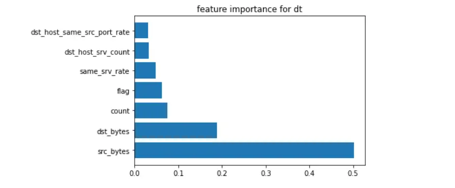

12. SKLearn Gradient Boosting Model

This code implements a Gradient Boosting Classifier using the scikit-learn library.

It initializes a GradientBoostingClassifier with a specified random seed (42), fits the model to the training data (x_train and y_train), and then evaluates its performance on both the training and test sets.

The training score indicates that the model achieved approximately 99.6% accuracy on the training data, while the testing score is around 99.3%, suggesting a high level of predictive accuracy and generalization.

Gradient Boosting is an ensemble learning technique that combines the predictions of multiple weak learners (typically decision trees) to create a robust and accurate predictive model.

The results suggest that the Gradient Boosting model performs well on the given dataset, capturing complex relationships between features and the target variable.

SKGB = GradientBoostingClassifier(random_state=42)
SKGB.fit(x_train, y_train)

SKGB_train, SKGB_test = SKGB.score(x_train , y_train), SKGB.score(x_test , y_test)

print(f"Training Score: {SKGB_train}")
print(f"Test Score: {SKGB_test}")

13. XGBoost Gradient Boosting Model

This code implements a Gradient Boosting Classifier using the XGBoost library, a popular gradient boosting framework.

It initializes an XGBClassifier with the "binary:logistic" objective (indicating binary classification) and a specified random seed (42).

The model is then fitted to the training data (x_train and y_train). The training and testing scores are subsequently calculated, revealing that the XGBoost model achieved perfect accuracy of 100% on the training data and an impressive accuracy of approximately 99.6% on the test data.

XGBoost is known for its efficiency and effectiveness in handling complex datasets, and in this case, it demonstrates strong predictive performance, capturing intricate patterns and relationships within the dataset.

The perfect training score suggests a potential risk of overfitting, and further fine-tuning or regularization may be considered for optimization.

xgb_model = XGBClassifier(objective="binary:logistic", random_state=42)
xgb_model.fit(x_train, y_train)

xgb_train, xgb_test = xgb_model.score(x_train , y_train), xgb_model.score(x_test , y_test)

print(f"Training Score: {xgb_train}")
print(f"Test Score: {xgb_test}")

14. Light Gradient Boosting Model

This code implements a Light Gradient Boosting Machine (LightGBM) classifier using the LGBMClassifier from the LightGBM library.

It initializes the model with a specified random seed (42) and fits it to the training data (x_train and y_train).

The training and testing scores are then calculated, revealing that the LightGBM model achieved a perfect accuracy of 100% on the training data and an impressive accuracy of approximately 99.5% on the test data.

LightGBM is known for its efficiency in handling large datasets and its ability to provide fast and accurate predictions.

The perfect training score suggests a potential risk of overfitting, and further fine-tuning or regularization may be considered for optimization.

Overall, the results indicate strong predictive performance on the given dataset.

lgb_model = LGBMClassifier(random_state=42)
lgb_model.fit(x_train, y_train)

lgb_train, lgb_test = lgb_model.score(x_train , y_train), lgb_model.score(x_test , y_test)

print(f"Training Score: {lgb_train}")
print(f"Test Score: {lgb_test}")

15. SKLearn AdaBoost Model

This code implements an AdaBoost classifier using the AdaBoostClassifier from scikit-learn. It initializes the model with a specified random seed (42) and fits it to the training data (x_train and y_train).

The training and testing scores are then calculated, indicating that the AdaBoost model achieved an accuracy of approximately 98.6% on the training data and a similar accuracy of around 98.6% on the test data.

AdaBoost is an ensemble learning technique that combines the predictions of weak learners (typically decision trees) to create a strong classifier.

The results suggest good predictive performance on both the training and testing sets, demonstrating the ability of AdaBoost to generalize well to unseen data.

ab_model = AdaBoostClassifier(random_state=42)

ab_model.fit(x_train, y_train)

ab_train, ab_test = ab_model.score(x_train , y_train), ab_model.score(x_test , y_test)

print(f"Training Score: {ab_train}")
print(f"Test Score: {ab_test}")

16. CatBoost Classifier Model

This implements a CatBoost Classifier using the CatBoostClassifier from the CatBoost library.

The model is initialized with verbosity set to 0 (silent mode), and it is fitted to the training data.

The training and testing scores are then calculated, revealing that the CatBoost model achieved an impressive accuracy of approximately 99.9% on the training data and approximately 99.5% on the test data.
CatBoost is a gradient-boosting algorithm that is particularly effective in handling categorical features and providing high-quality predictions.

The results suggest excellent predictive performance on the given dataset, demonstrating the strength of CatBoost in capturing complex relationships and patterns within the data.

cb_model = CatBoostClassifier(verbose=0)

cb_model.fit(x_train, y_train)

cb_train, cb_test = cb_model.score(x_train , y_train), cb_model.score(x_test , y_test)

print(f"Training Score: {cb_train}")
print(f"Test Score: {cb_test}")

17. Naive Bayes Model

This code implements a Naive Bayes classifier specifically using the Bernoulli Naive Bayes model (BernoulliNB) from scikit-learn.

The model is initialized, fitted to the training data (x_train and y_train), and subsequently evaluated on both the training and test sets.

The results indicate that the Bernoulli Naive Bayes model achieved an accuracy of approximately 89.6% on the training data and a similar accuracy of around 89.7% on the test data.

Bernoulli Naive Bayes is well-suited for binary and sparse feature datasets, and the accuracy scores suggest a reasonable level of predictive performance.

However, the model's performance may be influenced by its underlying assumption of features being binary, which might not be ideal for all types of datasets.

BNB_model = BernoulliNB()
BNB_model.fit(x_train, y_train)

BNB_train, BNB_test = BNB_model.score(x_train , y_train), BNB_model.score(x_test , y_test)

print(f"Training Score: {BNB_train}")
print(f"Test Score: {BNB_test}")

18. Voting Model

This code implements a Voting Classifier, an ensemble learning technique that combines the predictions of multiple individual models to make a final decision.

The VotingClassifier is constructed with a list of base models, including K Nearest Neighbors (KNN), XGBoost, Random Forest, Decision Tree, LightGBM, AdaBoost, and CatBoost.

The 'hard' voting strategy is used, meaning the final prediction is determined by a majority vote among the individual models. The Voting Classifier is then fitted to the training data (x_train and y_train), and its training and testing scores are calculated.

The results show the accuracy of the ensemble model on both datasets, providing an aggregated performance measure based on the diverse predictions of its constituent models. This approach aims to improve overall predictive performance and robustness by leveraging the strengths of different algorithms.

v_clf = VotingClassifier(estimators=[('KNeighborsClassifier', KNN_model), ("XGBClassifier", xgb_model), ("RandomForestClassifier", rf), ("DecisionTree", dt), ("XGBoost", xgb_model), ("LightGB", lgb_model), ("AdaBoost", ab_model), ("Catboost", cb_model)], voting = "hard")

v_clf.fit(x_train, y_train)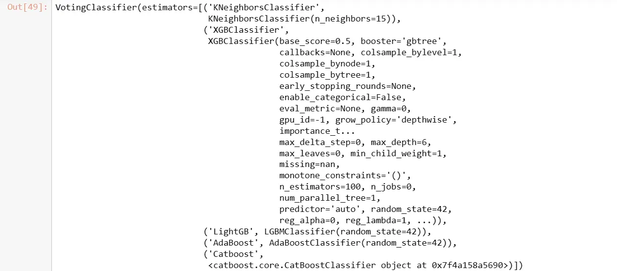

voting_train, voting_test = v_clf.score(x_train , y_train), v_clf.score(x_test , y_test)

print(f"Training Score: {voting_train}")
print(f"Test Score: {voting_test}")

19. SVM Model

This code performs hyperparameter optimization for a Support Vector Machine (SVM) classifier using Optuna.

The objective function defines a search space for SVM hyperparameters, including the choice of kernel ('linear', 'rbf', 'poly', 'linearSVC'), the regularization parameter 'C', and, for the 'poly' kernel, the polynomial degree.

The study aims to maximize accuracy on the test set over 30 trials. After optimization, the best trial's parameters are retrieved, and an SVM model is trained and evaluated on the provided dataset.

The results indicate that the SVM model, with an 'rbf' kernel and 'C' parameter set to 1.0, achieved an accuracy of approximately 96.3% on the training data and approximately 96.3% on the test data.

SVMs are known for their versatility in handling various data types, and the optimization process helps identify suitable hyperparameters for optimal performance on the given dataset.

def objective(trial):
    kernel = trial.suggest_categorical('kernel', ['linear', 'rbf', 'poly', 'linearSVC'])
    c = trial.suggest_float('c', 0.02, 1.0, step=0.02)
    if kernel in ['linear', 'rbf']:
        classifier_obj = SVC(kernel=kernel, C=c).fit(x_train, y_train)
    elif kernel == 'linearSVC':
        classifier_obj = LinearSVC(C=c).fit(x_train, y_train)
    elif kernel == 'poly':
        degree = trial.suggest_int('degree', 2, 10)
        classifier_obj = SVC(kernel=kernel, C=c, degree=degree).fit(x_train, y_train)
        
    accuracy = classifier_obj.score(x_test, y_test)
    return accuracy

study_svm = optuna.create_study(direction='maximize')
study_svm.optimize(objective, n_trials=30)
print(study_svm.best_trial)

if study_svm.best_trial.params['kernel'] in ['linear', 'rbf']:
    SVM_model = SVC(kernel=study_svm.best_trial.params['kernel'], C=study_svm.best_trial.params['c'])
elif kernel == 'linearSVC':
    SVM_model = LinearSVC(C=study_svm.best_trial.params['c'])
elif kernel == 'poly':
    SVM_model = SVC(kernel=study_svm.best_trial.params['kernel'], C=study_svm.best_trial.params['c'], degree=study_svm.best_trial.params['degree'])

SVM_model.fit(x_train, y_train)

SVM_train, SVM_test = SVM_model.score(x_train , y_train), SVM_model.score(x_test , y_test)

print(f"Training Score: {SVM_train}")
print(f"Test Score: {SVM_test}")

20. Summary

This code creates a tabular representation of the training and testing scores for various machine learning models.

The 'data' list contains model names along with their corresponding training and testing scores.

The tabulate function from the tabulate library is then used to format and print this information in a visually appealing grid.

The table includes scores for models such as K Nearest Neighbors (KNN), Logistic Regression, Decision Tree, Random Forest, Gradient Boosting Machine (GBM), XGBoost (XGBM), AdaBoost, LightGBM, CatBoost, Naive Bayes, Voting Classifier, and Support Vector Machine (SVM).

This presentation allows for a quick comparison of the performance of different models on the training and testing datasets, aiding in the assessment of their effectiveness and generalization capabilities.

data = [["KNN", KNN_train, KNN_test], 
        ["Logistic Regression", lg_train, lg_test],
        ["Decision Tree", dt_train, dt_test], 
        ["Random Forest", rf_train, rf_test], 
        ["GBM", SKGB_train, SKGB_test], 
        ["XGBM", xgb_train, xgb_test], 
        ["Adaboost", ab_train, ab_test], 
        ["light GBM", lgb_train, lgb_test],
        ["CatBoost", cb_train, cb_test], 
        ["Naive Baye Model", BNB_train, BNB_test], 
        ["Voting", voting_train, voting_test],
        ["SVM", SVM_train, SVM_test]]

col_names = ["Model", "Train Score", "Test Score"]
print(tabulate(data, headers=col_names, tablefmt="fancy_grid"))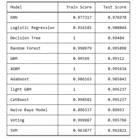

Conclusion

This beginner-friendly guide serves as a stepping stone for anyone eager to delve into the fascinating realm of Network Intrusion Detection.

We navigated through essential machine learning concepts, explored diverse models, and harnessed the power of NLP to fortify our defense against cyber threats.

For aspiring machine learning enthusiasts, this journey equips you with foundational knowledge and practical skills.

Product managers gain insights into bolstering network security, while researchers find a valuable resource for advancing intrusion detection systems.

As technology evolves, so do security challenges. By embracing the principles outlined in this guide, we empower ourselves to stay one step ahead in safeguarding networks against potential intrusions.

Let this guide be a catalyst for continuous learning and innovation in the ever-evolving field of cybersecurity.

Frequently Asked Questions

1. Are anomaly-based network intrusion detection systems effective in detecting network attacks?

Anomaly-based Network Intrusion Detection Systems (NIDS) can be effective in detecting network attacks by identifying deviations from established baselines.

Unlike signature-based systems that rely on known patterns, anomaly detection observes normal network behavior and flags any deviations as potential threats.

This approach is particularly valuable for detecting previously unknown attacks or zero-day exploits.

However, the effectiveness of anomaly-based NIDS relies heavily on accurately defining normal network behavior, minimizing false positives, and adapting to dynamic environments.

Continuous refinement and optimization are crucial to ensuring the reliability and efficiency of anomaly-based NIDS in the ever-evolving landscape of cyber threats.

2. How machine learning is used to detect malicious network traffic?

Machine learning plays a pivotal role in detecting malicious network traffic by leveraging advanced algorithms to analyze patterns, anomalies, and behaviors within network data.

Supervised learning models, such as decision trees and support vector machines, can be trained on labeled datasets to distinguish between normal and malicious traffic based on identified features.

Unsupervised learning, including clustering and anomaly detection algorithms, enables the system to identify irregular patterns without prior labeling.

Deep learning models, particularly neural networks, excel at extracting intricate features from large datasets, enhancing the system's ability to recognize complex threats.

The continuous learning capability of machine learning models allows them to adapt to evolving attack tactics, providing a dynamic and proactive defense against various cyber threats in the ever-changing landscape of network security.

3. Can ML models detect network traffic anomalies?

Yes, machine learning (ML) models excel at detecting network traffic anomalies by leveraging advanced algorithms to discern patterns and identify deviations from established norms.

These models, particularly unsupervised learning algorithms, can analyze vast amounts of network data and recognize unusual patterns that may indicate malicious activity.

By training on historical data and learning the baseline of normal network behavior, ML models can dynamically adapt to changes and swiftly identify anomalies, providing a proactive approach to detecting potential security threats.

This ability to analyze and understand complex relationships within network traffic sets ML apart as a powerful tool in anomaly detection, contributing significantly to the overall effectiveness of network intrusion detection systems.

Looking for high quality training data to train your vision/NLP model? Talk to our team to get a tool demo.