Annotated Data to Model Training with AWS Sage Maker: A Guide for Model Training

Introduction

This blog aims to delve into data annotation for training guidance within the AWS ecosystem. Whether or not you're familiar with AWS, we've got you covered, starting from the basics. In the realm of supervised machine learning (ML), labels signify values that a model is expected to learn and predict. The process of obtaining accurate labels involves either real-time recording or offline data annotation—tasks that assign labels to the dataset based on human intelligence.

However, manual dataset annotation proves to be a laborious and exhausting task for humans, particularly when dealing with large datasets. Even with labels that may seem obvious, the process remains error-prone due to human fatigue. Consequently, constructing training datasets consumes a significant chunk, up to 80%, of a data scientist's time. Addressing this challenge necessitates human intervention for the manual labeling of datasets, making it the most time-consuming aspect. Before diving into the details, let's familiarize ourselves with the platforms we'll be working on: Amazon S3 and SageMaker.

Understanding Amazon S3

Amazon S3 stands as a scalable, durable, and available object storage service equipped with a range of security features and cost-effective storage classes. Its versatility extends to applications such as storing static websites, hosting large files, managing backups, and serving data for big data analytics and machine learning.

The Significance of AWS SageMaker

Amazon SageMaker emerges as a fully managed service, empowering developers and data scientists to expedite the building, training, and deployment of machine learning (ML) models. SageMaker efficiently handles the intricacies of each step in the machine-learning process, simplifying the development of high-quality models.

SageMaker has the capability to build models trained by data stored in S3 buckets or sourced from a streaming data source like Kinesis shards. Once the models are trained, SageMaker streamlines the deployment process, making it seamless to transition them into production.

Data annotation:

In the realm of machine learning, data annotation is the pivotal process of labeling data to indicate the anticipated outcome that your machine learning model is meant to predict. It involves marking—labeling, tagging, transcribing, or processing—a dataset with the features you want your machine learning system to recognize. The ultimate goal is for your deployed model to autonomously recognize these features and make informed decisions or take actions accordingly.

Choosing the Optimal Algorithm for Your Use Case: Object Detection

Taking object detection as our focal point, selecting the right algorithm hinges on various factors, such as desired accuracy, speed, and computational resources. Below, we explore some of the most prominent object detection algorithms, along with their respective strengths and weaknesses.

Faster R-CNN (Region-based Convolutional Neural Network):

Advantages:

• Good accuracy.
• Two-stage architecture with a region proposal network (RPN) for improved localization.

Considerations:

• Can be computationally intensive.
• May not be as fast as some newer models for real-time applications.

YOLO (You Only Look Once):

Advantages:

• Fast and efficient, suitable for real-time applications.
• Single-stage architecture, making it simpler and faster than two-stage detectors.

Considerations:

• May sacrifice some accuracy compared to slower, two-stage detectors.
• YOLOv3 and later versions have improved accuracy.

SSD (Single Shot Multibox Detector):

Advantages:

• Balances speed and accuracy.
• Single-stage architecture, making it faster than Faster R-CNN.
• Good performance on small objects.

Considerations:

• May not be as accurate as two-stage detectors like Faster R-CNN.
• Can have more false positives compared to other models.

Importance of Data Labeling:

1. Providing Ground Truth: Data labels act as the "ground truth" against which machine learning models are assessed. By comparing the model's predictions to the labelled data, we can gauge its accuracy and pinpoint areas for improvement. High-quality labeling ensures that the model learns from accurate and consistent information.

2. Enabling Supervised Learning: Supervised learning, a prevalent machine learning approach, relies on labelled data to train models. By furnishing examples of inputs and their corresponding outputs, data labeling empowers the model to discern patterns and relationships within the data. This proves critical for tasks such as image classification, speech recognition, and sentiment analysis.

3. Improving Model Performance: The precision of data labeling directly influences model performance. The more accurate and consistent the labels, the more reliable the model's predictions become. Poor-quality labelling introduces noise and inconsistencies into the training data, leading to inaccurate or biased predictions.

Annotating Data with AWS Ground Truth for bird Classification

To kickstart our journey, we will commence by annotating the data using AWS Ground Truth, ensuring that we obtain meticulously labelled datasets. In this instance, let's focus on the task of building a model for classifying birds. Our goal is to acquire data where the bird is distinctly highlighted in the image. This will be achieved by leveraging the annotation services offered by AWS Ground Truth.

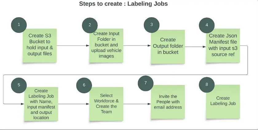
Step 0: Create an S3 bucket, upload images, and generate manifest files.

{"source-ref": "s3://bucket-input/input/image1.jpeg"} 
{"source-ref": "s3://bucket-input/input/image2.jpeg"} 
{"source-ref": "s3://bucket-input/input/image3.jpeg"} 
{"source-ref": "s3://bucket-input/input/image4.jpeg"} 

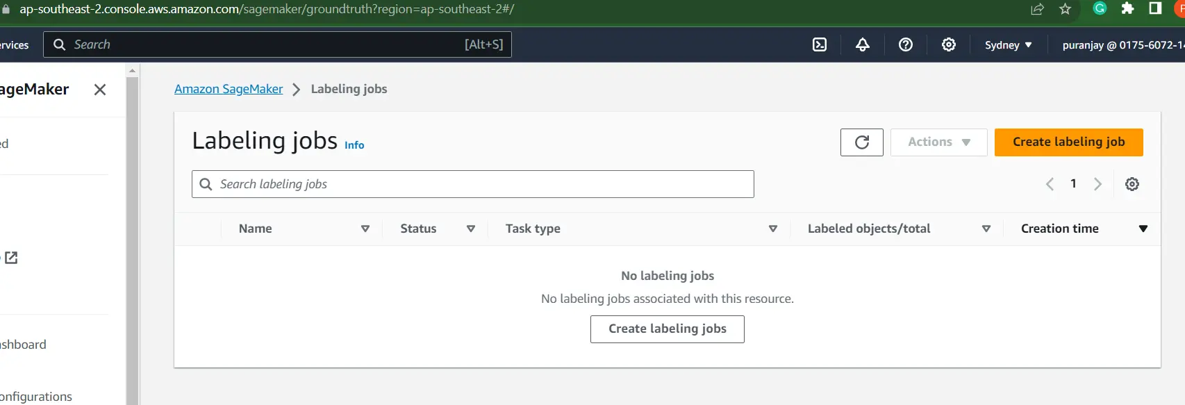
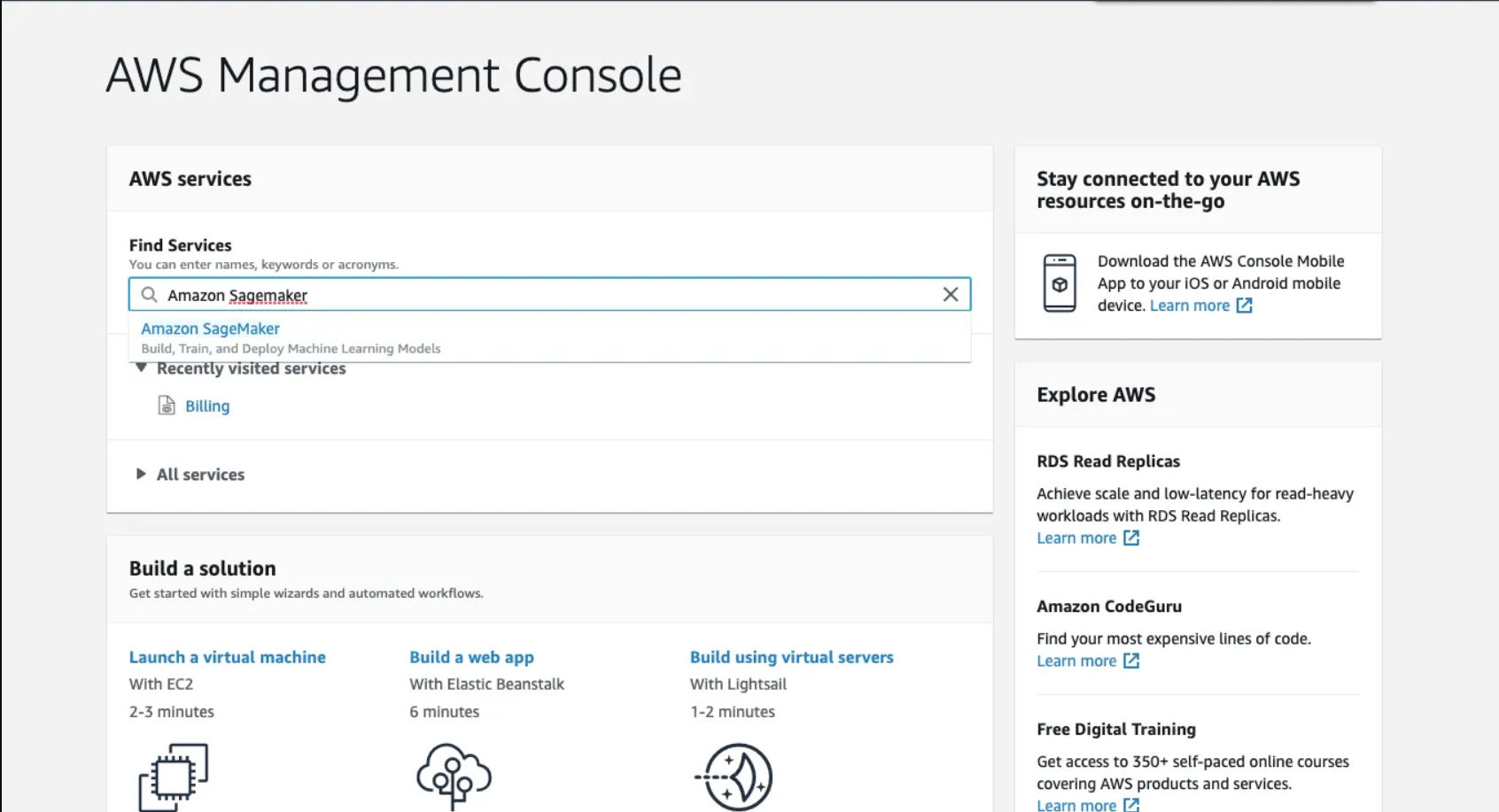
Step 1: In the AWS console, search for AWS SageMaker, and then navigate to Labeling Jobs/Ground Truth. Here, you can label your images by clicking on Create Labeling Job.

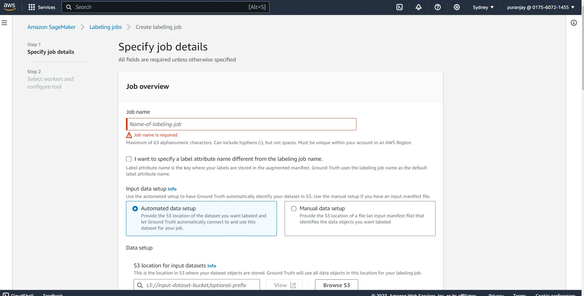
Step 2: Fill out the Job name and your bucket URL where your data is stored.

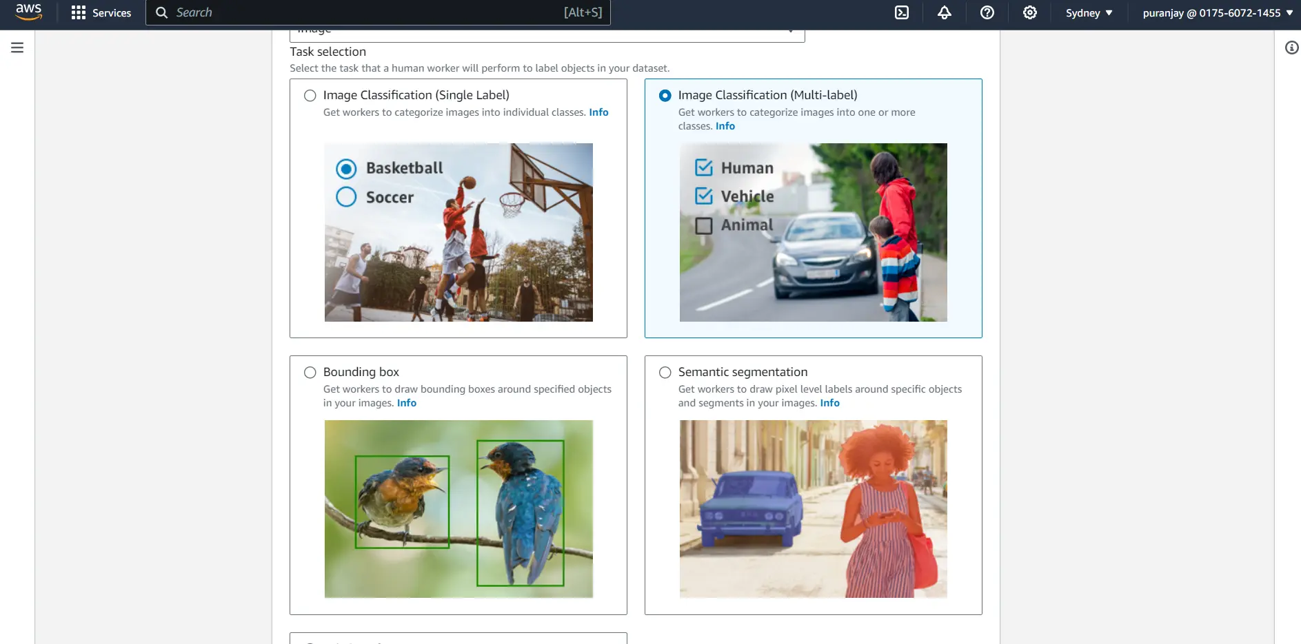
Step 3: Select the task type based on your use case, whether you require a single class label, multi-class label, semantic segmentation, or bounding box.

Step 4: Label your image with the tools mentioned below, and you can label multiple images to create your own dataset.

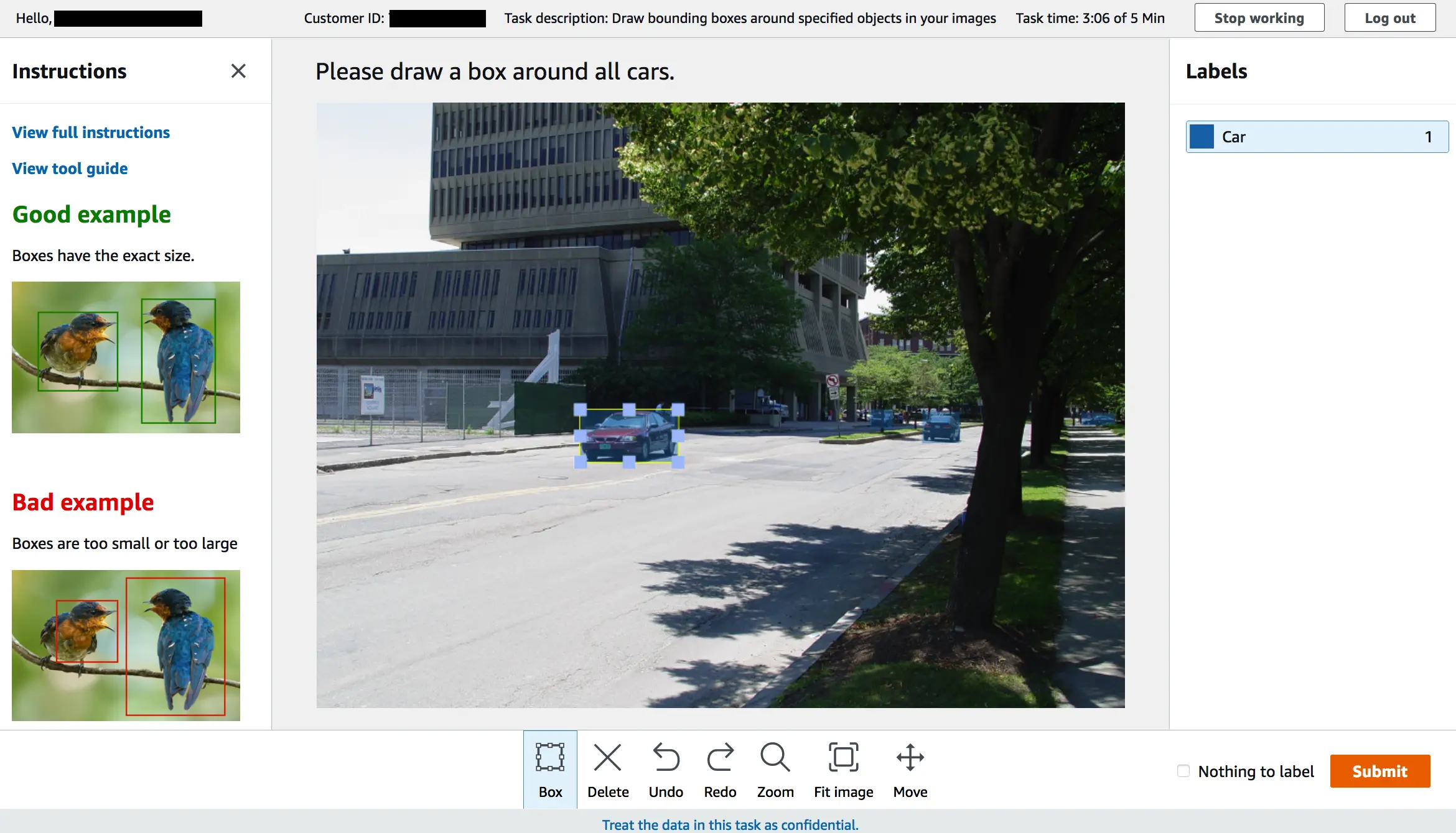
Annotated images are visible directly in the AWS console, which comes in handy for sanity checks. You can also click on any image and see the list of labels that have been applied. Our main purpose is to use this information to train machine learning models, and you can find this data in your bucket.

Disadvantages of AWS ground truth

However, for large datasets, Amazon AWS does not provide support for collaboration and better annotation tools. As a result, many individuals opt to outsource a labeling platform that offers automated labeling, faster manual labeling, and collaborative annotation.

This enables the division of labeling tasks among multiple individuals, significantly accelerating the labeling process—nearly 90 times faster than the traditional approach.

Labellerr Helps Getting Large Volume Labels

This tool addresses all the disadvantages mentioned above in Ground Truth, significantly accelerating the annotation process for all images.

Additionally, after annotating all the images, it can export them to your desired cloud service, whether it's AWS, Azure, or Google Cloud. Now that you have all the annotated images, and you want to write code for model training, let's follow the steps below to start training your model.

First, let's set up AWS SageMaker!

step 1: Go to AWS, management console

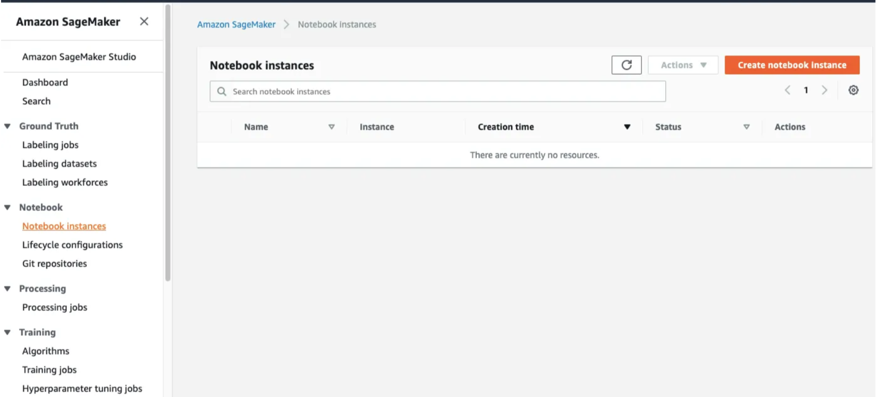
Step 2: Open the Notebook Instances and click on Create Notebook Instance.

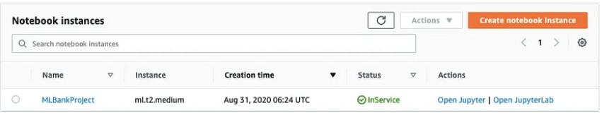
• During the setup, you'll encounter prompts for Notebook Instance Settings. Provide it with a descriptive name and opt for the ml.t2.medium instance type. This represents the basic tier and is suitable for our current needs. As we delve into more advanced models, we can consider higher-tier instances. Cost considerations need not be a concern, as AWS operates on a pay-per-use pricing model, ensuring you only pay for the resources you consume.

Other services can be left to their default settings. If you wish to explore them further, you can always refer to the documentation for more detailed information. documentation

Step 3: Create an IAM role

Step 4: Confirmation screen

After this, you will receive a message saying

success! you created an IAM role.

After some time after loading, we can see the console says the notebook instance is in "Inservice"

Step 5: Create a new file and select.ipynb file from the drop-down menu

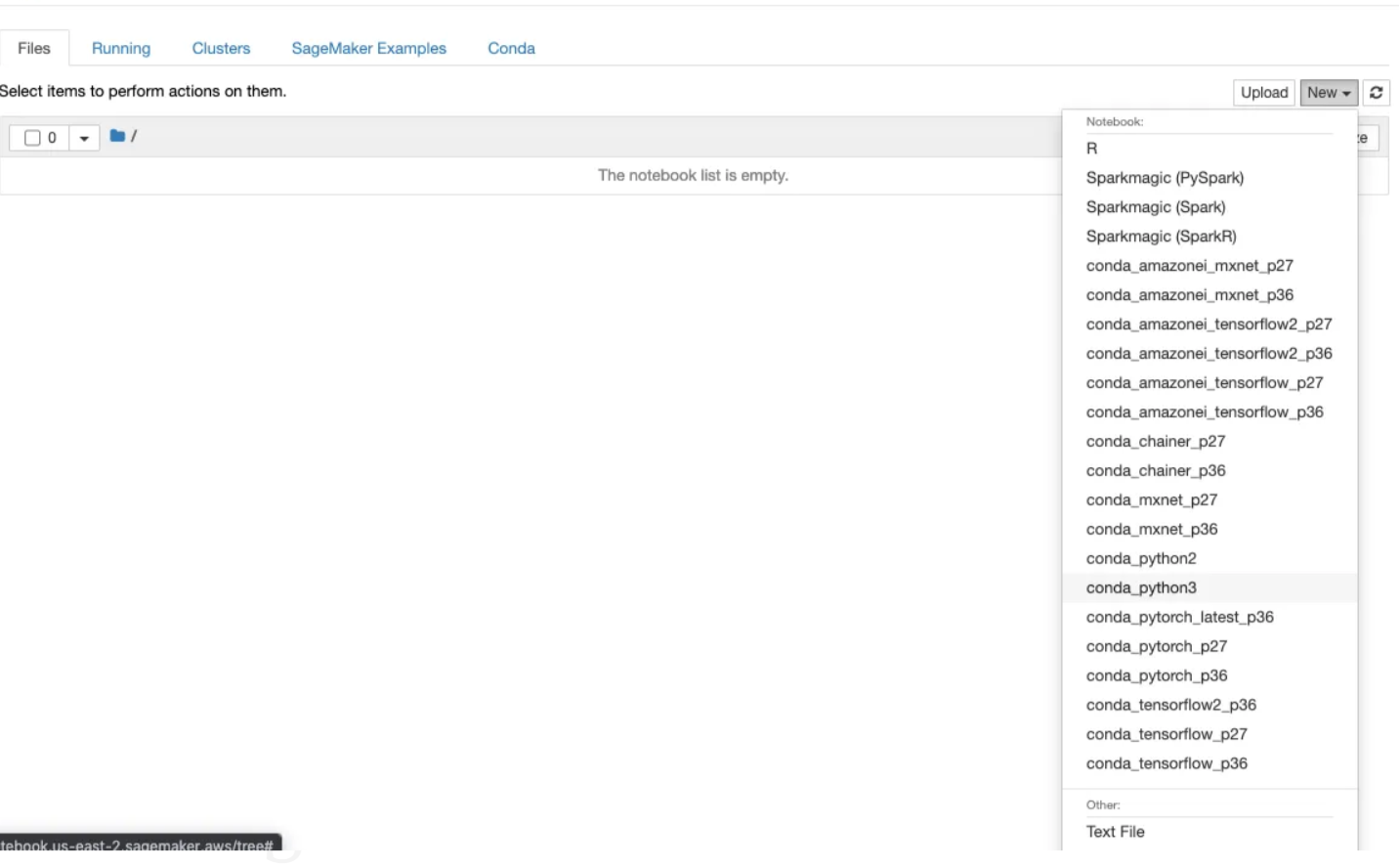
Now that our environment setup is complete, let's dive into coding. For this exercise, we'll focus on object detection for bird species using the Bird Species dataset. You can find this dataset here in Bird Species Dataset.

Step 0: Setup

! pip install distro
import distro
if "debian" in distro.linux_distribution()[0].lower():
    ! apt-get update
    ! apt-get install ffmpeg libsm6 libxext6  -y

import sys

!{sys.executable} -m pip install opencv-python
!{sys.executable} -m pip install mxnet

Step 1: Code for Retrieving Default S3 Bucket and Prefix in SageMaker

In the following code snippet, our objective is to identify the S3 bucket designated for the provision of training and validation datasets. Furthermore, this bucket will serve as the repository for storing the trained model artifacts. Although a customized bucket is utilized in this notebook, it is essential to recognize that a default session bucket is a feasible alternative. To augment the organization of the bucket content, an object prefix is employed.

import sagemaker

bucket = sagemaker.Session().default_bucket()
prefix = "DEMO-ObjectDetection-birds"

print("s3://{}/{}/".format(bucket, prefix))

Step 2: Set up and authenticate the use of AWS services.

from sagemaker import get_execution_role

role = get_execution_role()
print(role)
sess = sagemaker.Session()

step 3: Download and unpack the dataset

import os
import urllib.request


def download(url):
    filename = url.split("/")[-1]
    if not os.path.exists(filename):
        urllib.request.urlretrieve(url, filename)
%%time
# download('http://www.vision.caltech.edu/visipedia-data/CUB-200-2011/CUB_200_2011.tgz')
# CalTech's download is (at least temporarily) unavailable since August 2020.

# Can now use one made available by fast.ai .
download("https://s3.amazonaws.com/fast-ai-imageclas/CUB_200_2011.tgz")

step 4: Unpacking and removing tar files

%%time
# Clean up prior version of the downloaded dataset if you are running this again
!rm -rf CUB_200_2011

# Unpack and then remove the downloaded compressed tar file
!gunzip -c ./CUB_200_2011.tgz | tar xopf -
!rm CUB_200_2011.tgz

step 5: Defining the parameters

import pandas as pd
import cv2
import boto3
import json

runtime = boto3.client(service_name="runtime.sagemaker")

import matplotlib.pyplot as plt

%matplotlib inline

RANDOM_SPLIT = False
SAMPLE_ONLY = True
FLIP = False

# To speed up training and experimenting, you can use a small handful of species.
# To see the full list of the classes available, look at the content of CLASSES_FILE.
CLASSES = [17, 36, 47, 68, 73]

# Otherwise, you can use the full set of species
if not SAMPLE_ONLY:
    CLASSES = []
    for c in range(200):
        CLASSES += [c + 1]

RESIZE_SIZE = 256

BASE_DIR = "CUB_200_2011/"
IMAGES_DIR = BASE_DIR + "images/"

CLASSES_FILE = BASE_DIR + "classes.txt"
BBOX_FILE = BASE_DIR + "bounding_boxes.txt"
IMAGE_FILE = BASE_DIR + "images.txt"
LABEL_FILE = BASE_DIR + "image_class_labels.txt"
SIZE_FILE = BASE_DIR + "sizes.txt"
SPLIT_FILE = BASE_DIR + "train_test_split.txt"

TRAIN_LST_FILE = "birds_ssd_train.lst"
VAL_LST_FILE = "birds_ssd_val.lst"

if SAMPLE_ONLY:
    TRAIN_LST_FILE = "birds_ssd_sample_train.lst"
    VAL_LST_FILE = "birds_ssd_sample_val.lst"

TRAIN_RATIO = 0.8
CLASS_COLS = ["class_number", "class_id"]
IM2REC_SSD_COLS = [
    "header_cols",
    "label_width",
    "zero_based_id",
    "xmin",
    "ymin",
    "xmax",
    "ymax",
    "image_file_name",
]

step 6:Explore the dataset images

def show_species(species_id):
    _im_list = !ls $IMAGES_DIR/$species_id

    NUM_COLS = 6
    IM_COUNT = len(_im_list)

    print('Species ' + species_id + ' has ' + str(IM_COUNT) + ' images.')
    
    NUM_ROWS = int(IM_COUNT / NUM_COLS)
    if ((IM_COUNT % NUM_COLS) > 0):
        NUM_ROWS += 1

    fig, axarr = plt.subplots(NUM_ROWS, NUM_COLS)
    fig.set_size_inches(8.0, 16.0, forward=True)

    curr_row = 0
    for curr_img in range(IM_COUNT):
        # fetch the url as a file type object, then read the image
        f = IMAGES_DIR + species_id + '/' + _im_list[curr_img]
        a = plt.imread(f)

        # find the column by taking the current index modulo 3
        col = curr_img % NUM_ROWS
        # plot on relevant subplot
        axarr[col, curr_row].imshow(a)
        if col == (NUM_ROWS - 1):
            # we have finished the current row, so increment row counter
            curr_row += 1

    fig.tight_layout()       
    plt.show()
        
    # Clean up
    plt.clf()
    plt.cla()
    plt.close()

step 7: Checking the output of the class

classes_df = pd.read_csv(CLASSES_FILE, sep=" ", names=CLASS_COLS, header=None)
criteria = classes_df["class_number"].isin(CLASSES)
classes_df = classes_df[criteria]
print(classes_df.to_csv(columns=["class_id"], sep="\t", index=False, header=False))
show_species("017.Cardinal")

Step 8: Generate the record IO files

For this specific dataset, bounding box annotations are specified in absolute terms. The RecordIO format, however, necessitates them to be defined in terms relative to the image size. The subsequent code iterates through each image, extracts the height and width, and stores this information in a file for future use. It's worth noting that certain publicly available datasets already offer such a file explicitly for this purpose.

%%time
SIZE_COLS = ["idx", "width", "height"]


def gen_image_size_file():
    print("Generating a file containing image sizes...")
    images_df = pd.read_csv(
        IMAGE_FILE, sep=" ", names=["image_pretty_name", "image_file_name"], header=None
    )
    rows_list = []
    idx = 0
    image_file_name = images_df["image_file_name"].dropna(axis=0)
    for i in image_file_name:
        # TODO: add progress bar
        idx += 1
        img = cv2.imread(IMAGES_DIR + i)
        dimensions = img.shape
        height = img.shape[0]
        width = img.shape[1]
        image_dict = {"idx": idx, "width": width, "height": height}
        rows_list.append(image_dict)

    sizes_df = pd.DataFrame(rows_list)
    print("Image sizes:\n" + str(sizes_df.head()))

    sizes_df[SIZE_COLS].to_csv(SIZE_FILE, sep=" ", index=False, header=None)


gen_image_size_file()

step 9: Generate a list of producing recordIO files.

def split_to_train_test(df, label_column, train_frac=0.8):
    train_df, test_df = pd.DataFrame(), pd.DataFrame()
    labels = df[label_column].unique()
    for lbl in labels:
        lbl_df = df[df[label_column] == lbl]
        lbl_train_df = lbl_df.sample(frac=train_frac)
        lbl_test_df = lbl_df.drop(lbl_train_df.index)
        print(
            "\n{}:\n---------\ntotal:{}\ntrain_df:{}\ntest_df:{}".format(
                lbl, len(lbl_df), len(lbl_train_df), len(lbl_test_df)
            )
        )
        train_df = train_df.append(lbl_train_df)
        test_df = test_df.append(lbl_test_df)
    return train_df, test_df


def gen_list_files():
    # use generated sizes file
    sizes_df = pd.read_csv(
        SIZE_FILE, sep=" ", names=["image_pretty_name", "width", "height"], header=None
    )
    bboxes_df = pd.read_csv(
        BBOX_FILE,
        sep=" ",
        names=["image_pretty_name", "x_abs", "y_abs", "bbox_width", "bbox_height"],
        header=None,
    )
    split_df = pd.read_csv(
        SPLIT_FILE, sep=" ", names=["image_pretty_name", "is_training_image"], header=None
    )
    print(IMAGE_FILE)
    images_df = pd.read_csv(
        IMAGE_FILE, sep=" ", names=["image_pretty_name", "image_file_name"], header=None
    )
    print("num images total: " + str(images_df.shape[0]))
    image_class_labels_df = pd.read_csv(
        LABEL_FILE, sep=" ", names=["image_pretty_name", "class_id"], header=None
    )

    # Merge the metadata into a single flat dataframe for easier processing
    full_df = pd.DataFrame(images_df)
    full_df.reset_index(inplace=True)
    full_df = pd.merge(full_df, image_class_labels_df, on="image_pretty_name")
    full_df = pd.merge(full_df, sizes_df, on="image_pretty_name")
    full_df = pd.merge(full_df, bboxes_df, on="image_pretty_name")
    full_df = pd.merge(full_df, split_df, on="image_pretty_name")
    full_df.sort_values(by=["index"], inplace=True)

    # Define the bounding boxes in the format required by SageMaker's built in Object Detection algorithm.
    # the xmin/ymin/xmax/ymax parameters are specified as ratios to the total image pixel size
    full_df["header_cols"] = 2  # one col for the number of header cols, one for the label width
    full_df["label_width"] = 5  # number of cols for each label: class, xmin, ymin, xmax, ymax
    full_df["xmin"] = full_df["x_abs"] / full_df["width"]
    full_df["xmax"] = (full_df["x_abs"] + full_df["bbox_width"]) / full_df["width"]
    full_df["ymin"] = full_df["y_abs"] / full_df["height"]
    full_df["ymax"] = (full_df["y_abs"] + full_df["bbox_height"]) / full_df["height"]

    # object detection class id's must be zero based. map from
    # class_id's given by CUB to zero-based (1 is 0, and 200 is 199).

    if SAMPLE_ONLY:
        # grab a small subset of species for testing
        criteria = full_df["class_id"].isin(CLASSES)
        full_df = full_df[criteria]

    unique_classes = full_df["class_id"].drop_duplicates()
    sorted_unique_classes = sorted(unique_classes)

    id_to_zero = {}
    i = 0.0
    for c in sorted_unique_classes:
        id_to_zero[c] = i
        i += 1.0

    full_df["zero_based_id"] = full_df["class_id"].map(id_to_zero)

    full_df.reset_index(inplace=True)

    # use 4 decimal places, as it seems to be required by the Object Detection algorithm
    pd.set_option("display.precision", 4)

    train_df = []
    val_df = []

    if RANDOM_SPLIT:
        # split into training and validation sets
        train_df, val_df = split_to_train_test(full_df, "class_id", TRAIN_RATIO)

        train_df[IM2REC_SSD_COLS].to_csv(TRAIN_LST_FILE, sep="\t", float_format="%.4f", header=None)
        val_df[IM2REC_SSD_COLS].to_csv(VAL_LST_FILE, sep="\t", float_format="%.4f", header=None)
    else:
        train_df = full_df[(full_df.is_training_image == 1)]
        train_df[IM2REC_SSD_COLS].to_csv(TRAIN_LST_FILE, sep="\t", float_format="%.4f", header=None)

        val_df = full_df[(full_df.is_training_image == 0)]
        val_df[IM2REC_SSD_COLS].to_csv(VAL_LST_FILE, sep="\t", float_format="%.4f", header=None)

    print("num train: " + str(train_df.shape[0]))
    print("num val: " + str(val_df.shape[0]))
    return train_df, val_df
train_df, val_df = gen_list_files()

Step 10: Convert the data into  RecordIo format

!tail -3 $TRAIN_LST_FILE
!python tools/im2rec.py --resize $RESIZE_SIZE --pack-label birds_ssd_sample $BASE_DIR/images/

step 11: Upload the record IO files to S3.

Upload the training and validation data to the S3 bucket. This process is executed through multiple channels, which are essentially directories in the bucket that distinguish the types of data supplied to the algorithm. In the context of the object detection algorithm, these directories are named train and validation.

# Upload the RecordIO files to train and validation channels
train_channel = prefix + "/train"
validation_channel = prefix + "/validation"

sess.upload_data(path="birds_ssd_sample_train.rec", bucket=bucket, key_prefix=train_channel)
sess.upload_data(path="birds_ssd_sample_val.rec", bucket=bucket, key_prefix=validation_channel)

s3_train_data = "s3://{}/{}".format(bucket, train_channel)
s3_validation_data = "s3://{}/{}".format(bucket, validation_channel)

Step 12: Training the model

Subsequently, we specify an output location in S3 where the model artifacts will be deposited upon the completion of the training. These artifacts constitute the output of the algorithm's training job. Additionally, we obtain the URI for the Amazon SageMaker Object Detection Docker image. This ensures that the estimator utilizes the correct algorithm corresponding to the current region.

from sagemaker import image_uris

training_image = image_uris.retrieve(
    region=sess.boto_region_name, framework="object-detection", version="latest"
)
print(training_image
s3_output_location = "s3://{}/{}/output".format(bucket, prefix)
od_model = sagemaker.estimator.Estimator(
    training_image,
    role,
    instance_count=1,
    instance_type="ml.p3.2xlarge",
    volume_size=50,
    max_run=360000,
    input_mode="File",
    output_path=s3_output_location,
    sagemaker_session=sess,

step 13: Define the hyperparameters:

def set_hyperparameters(num_epochs, lr_steps):
    num_classes = classes_df.shape[0]
    num_training_samples = train_df.shape[0]
    print("num classes: {}, num training images: {}".format(num_classes, num_training_samples))

    od_model.set_hyperparameters(
        base_network="resnet-50",
        use_pretrained_model=1,
        num_classes=num_classes,
        mini_batch_size=16,
        epochs=num_epochs,
        learning_rate=0.001,
        lr_scheduler_step=lr_steps,
        lr_scheduler_factor=0.1,
        optimizer="sgd",
        momentum=0.9,
        weight_decay=0.0005,
        overlap_threshold=0.5,
        nms_threshold=0.45,
        image_shape=512,
        label_width=350,
        num_training_samples=num_training_samples,
    )
 set_hyperparameters(100, "33,67")

step 14: Defining the data channels

With the hyperparameters configured, we proceed to define the data channels to be passed to the algorithm. To achieve this, we create sagemaker.session.s3_input objects from our data channels. These objects are then organized into a straightforward dictionary, which the algorithm utilizes. It's worth noting that you have the option to include a third channel named model for incremental training, allowing you to continue training from where you left off with a prior model.

train_data = sagemaker.inputs.TrainingInput(
    s3_train_data,
    distribution="FullyReplicated",
    content_type="application/x-recordio",
    s3_data_type="S3Prefix",
)
validation_data = sagemaker.inputs.TrainingInput(
    s3_validation_data,
    distribution="FullyReplicated",
    content_type="application/x-recordio",
    s3_data_type="S3Prefix",
)
data_channels = {"train": train_data, "validation": validation_data}

step 15:Submit the training Job:

The training process encompasses several steps. Initially, the instances requested during the creation of the Estimator classes are provisioned and set up with the necessary libraries. Subsequently, the data from our channels is downloaded onto the instance. Once this preparatory phase is complete, the actual training process commences.

%%time
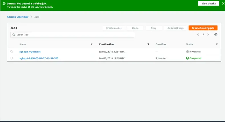
od_model.fit(inputs=data_channels, logs=True)

Step 16: Now that the training job is complete, you can observe it listed in the following manner.

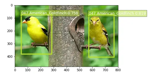
Host The model

After the training is successfully completed, we can deploy the trained model as an Amazon SageMaker real-time hosted endpoint. This deployment enables us to make predictions, also known as inferences, from the model.

%%time
object_detector = od_model.deploy(initial_instance_count=1, instance_type="ml.m5.xlarge")

Conclusion:

In summary, the outlined steps detail the procedure for preparing, training, and deploying a model through Amazon SageMaker. The process encompasses configuring and authenticating AWS services, transforming data into RecordIO format, and organizing it into distinct channels.

The resulting model artifacts are stored in an S3 bucket. Upon completing the training, the model is deployed as a real-time hosted endpoint, allowing for predictions or inferences. These steps provide a structured and effective approach to machine learning tasks within the AWS platform.