ML Guide To Build Credit Card Fraud Detection Model

Introduction

Credit card fraud has remained the most common type of identity theft through the first three quarters of 2023, with 318,000 reported cases.

This makes it a serious issue affecting millions worldwide. It leads to financial losses for both cardholders and financial institutions, as well as damages to trust and reputation in the financial system.

This blog aims to provide an overview of building a credit card fraud detection model using machine learning.

It will explore the importance of fraud detection, the challenges involved, and the role of machine learning algorithms in mitigating fraud risks in financial transactions.

Common Types of Fraud

Credit card fraud can take various forms, with fraudsters employing sophisticated techniques to exploit vulnerabilities in the system.

Traditional systems utilize rule-based approaches and anomaly detection to mitigate these risks.

To better understand the challenges faced in combating fraud, let's explore three prevalent types of credit card fraud and how traditional systems tackle them.

Counterfeit Card Fraud

Fraudsters clone legitimate credit cards or create counterfeit cards using stolen card information. Traditional systems use signature verification, EMV chip technology, and magnetic stripe analysis to detect counterfeit cards. Any deviation from the expected card characteristics triggers alerts for further investigation.

Card-Not-Present (CNP) Fraud

Fraudsters use stolen credit card details to make online or phone transactions where the physical card is not required.

Traditional systems employ address verification systems (AVS), card security codes (CVV/CVC), and transaction velocity checks to detect CNP fraud.

These systems flag transactions with mismatched or suspicious details for manual review.

Identity Theft

Fraudsters obtain personal information, such as social security numbers or passwords, to impersonate individuals and open fraudulent credit card accounts.

Traditional systems utilize knowledge-based authentication (KBA) or biometric verification, to confirm the identity of applicants. Additionally, credit monitoring services and fraud alerts are employed to detect suspicious account activities.

While traditional systems offer effective countermeasures, machine learning presents a dynamic approach capable of addressing evolving fraud patterns and enhancing detection accuracy.

Using machine learning

Machine learning can dynamically adapt to evolving fraud patterns and detect subtle anomalies that may not be captured by rule-based systems.

By continuously learning from new data, machine learning models can improve accuracy and reduce false positives.

AI-powered systems can analyze transactions in real-time, enabling immediate detection and response to fraudulent activities, reducing the impact of fraud on financial institutions and consumers.

AI facilitates the integration of diverse data sources, such as transaction history, customer behavior, and external threat intelligence.

Challenges

However, deploying machine learning models for fraud detection comes with its own set of challenges, including dealing with imbalanced data, thwarting adversarial attacks, and ensuring model interpretability.

Imbalanced Data: Credit card fraud datasets are often highly imbalanced, with fraudulent transactions representing a small fraction of the total data.

Imbalanced data can lead to biased models that prioritize accuracy on the majority class while neglecting the minority class, resulting in poor fraud detection performance.

Adversarial Attacks: Fraudsters continuously evolve their tactics to evade detection, including adversarial attacks aimed at fooling machine learning models.

Adversarial attacks involve subtly modifying input data to cause misclassification, undermining the effectiveness of fraud detection systems trained on historical data.

Interpretability :Understanding how these models make decisions is crucial for regulatory compliance and stakeholder trust, yet complex models may be perceived as "black boxes," making it challenging to interpret their outputs.

Steps for building a model

Understanding the Dataset

Importing the dataset

To import the Kaggle the credit card fraud detection dataset in the google collab environment first generate a new API token from account settings in Kaggle. A 'kaggle.json' file will be downloaded.

The kaggle file contains credentials corresponding to your account. Upload this file into the collab notebook.

Run the following commands in cells to directly import datasets in the collab environment.

! pip install kaggle
! mkdir ~/.kaggle
! cp kaggle.json ~/.kaggle/
! chmod 600 ~/.kaggle/kaggle.json

!kaggle datasets download -d mlg-ulb/creditcardfraud
!unzip creditcardfraud.zip

import pandas as pd 
df = pd.read_csv('creditcard.csv')

Exploratory Data Analysis

df.shape # results in (284807, 31)

df.columns 

'''['Time', 'V1', 'V2', 'V3', 'V4', 'V5', 'V6', 'V7', 'V8', 'V9', 'V10',
       'V11', 'V12', 'V13', 'V14', 'V15', 'V16', 'V17', 'V18', 'V19', 'V20',
       'V21', 'V22', 'V23', 'V24', 'V25', 'V26', 'V27', 'V28', 'Amount',
       'Class']'''

1. Time: The time elapsed between each transaction and the first transaction in the dataset (in seconds).
2. V1-V28: Anonymous features resulting from a PCA transformation for privacy reasons. These features likely represent different aspects of the transaction data, such as transaction amount, location, and time.
3. Amount: The transaction amount.
4. Class: The target variable indicating whether a transaction is fraudulent (1) or legitimate (0).

df['Class'].value_counts() #0    284315    1       492

We can use a histogram to visualize the distribution of our dataset.

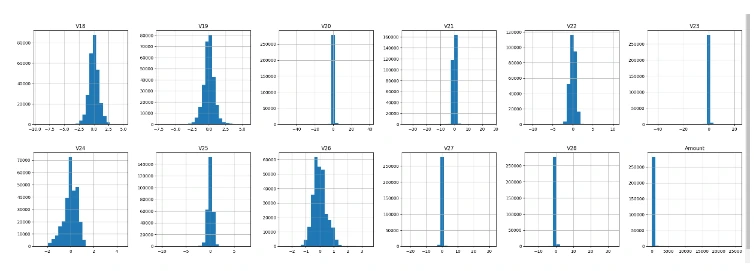
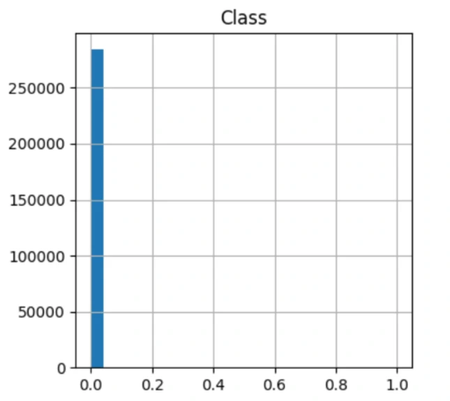
This result indicates that the dataset is extremely imbalanced. The model can get a bias as the fraud transactions are nearly negligible compared to the fair transactions.

Data Preprocessing

Scaling features is a crucial preprocessing step in machine learning pipelines.

Robust scaling is particularly useful when dealing with features that are sensitive to outliers, such as 'Amount' and 'Time' in credit card transaction data.Robust scaling is a preprocessing technique that scales the features to be robust to outliers by removing the median and scaling data according to the interquartile range.

from sklearn.preprocessing import RobustScaler

scaler = RobustScaler()
df[['Amount', 'Time']] = scaler.fit_transform(df[['Amount', 'Time']])

Next we code the process of balancing an imbalanced dataset by undersampling the majority class (non-fraud) to match the number of samples in the minority class (fraud). The dataset is shuffled to ensure randomness before and after undersampling.

df = df.sample(frac=1, random_state=42)
df

not_frauds = df[new_df['Class'] == 0]
frauds = df[new_df['Class'] == 1]

balanced_df = pd.concat([frauds, not_frauds.sample(n=len(frauds), random_state=42)])

balanced_df = balanced_df.sample(frac=1, random_state=42)

balanced_df['Class'].value_counts()

This code snippet splits the balanced dataset into training, testing, and validation sets using the `train_test_split'  function from Scikit-Learn. The dataset is first converted to a NumPy array, and then split into features (x) and labels (y).

The training set is further split into training and validation sets for model evaluation during training.

from sklearn.model_selection import train_test_split
balanced_df_np = balanced_df.to_numpy()


x_train_val_b, x_test_b, y_train_val_b, y_test_b = train_test_split(
    balanced_df_np[:, :-1], balanced_df_np[:, -1].astype(int), test_size=0.15, random_state=42
)
x_train_b, x_val_b, y_train_b, y_val_b = train_test_split(
    x_train_val_b, y_train_val_b, test_size=0.15, random_state=42
)


x_train_b.shape, y_train_b.shape, x_test_b.shape, y_test_b.shape, x_val_b.shape, y_val_b.shape

The ouput would be : ((710, 30), (710,), (148, 30), (148,), (126, 30), (126,))

Checking the class distribution:

pd.Series(y_train_b).value_counts(), pd.Series(y_test_b).value_counts(), pd.Series(y_val_b).value_counts()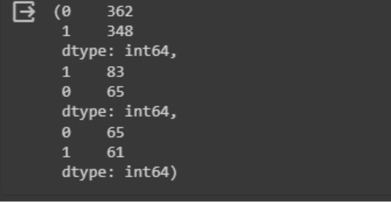

Building a Shallow Neural Network Model

Neural networks, including shallow ones, can capture complex patterns in data and are capable of learning non-linear relationships between features and labels.

By defining and training a shallow neural network model, we aim to leverage its expressive power to improve classification performance compared to traditional linear models like logistic regression.

The use of ReLU activation in the hidden layer introduces non-linearity, allowing the model to learn intricate patterns in the data.

Batch normalization helps stabilize and accelerate training by normalizing the input to each layer.

# Define the shallow neural network model
shallow_nn = Sequential()
shallow_nn.add(InputLayer(input_shape=(x_train_b.shape[1],)))  # Corrected input shape
shallow_nn.add(Dense(2, activation='relu'))  # Specify activation function
shallow_nn.add(BatchNormalization())
shallow_nn.add(Dense(1, activation='sigmoid'))  # Specify activation function

The ModelCheckpoint callback is used to save the best-performing model based on validation accuracy, ensuring that we retain the model with the optimal performance.

Finally, training the model on the training data and validating it on the validation data allows us to monitor its performance and adjust hyperparameters if necessary to improve generalization.

# Define the ModelCheckpoint callback to save the best model
checkpoint = ModelCheckpoint('shallow_nn', save_best_only=True)

# Compile the model
shallow_nn.compile(optimizer='adam', loss='binary_crossentropy', metrics=['accuracy'])

# Train the model
shallow_nn.fit(x_train_b, y_train_b, validation_data=(x_val_b, y_val_b), epochs=40, callbacks=[checkpoint])

Evaluating the performance

The purpose of this function is to generate binary predictions (0 or 1) from the output probabilities of the neural network model.

This is necessary for evaluating the performance of the model and comparing its predictions with the true class labels.

By applying a threshold of 0.5, instances with predicted probabilities above the threshold are classified as belonging to the positive class (Fraud), while instances with predicted probabilities below the threshold are classified as belonging to the negative class (Not Fraud).

def neural_net_predictions(model, x):
    return (model.predict(x).flatten() > 0.5).astype(int)

neural_net_predictions(shallow_nn_b, x_val_b)

These binary predictions can then be used to compute various classification metrics, such as precision, recall, and F1-score, using the classification_report function from Scikit-Learn.

from sklearn.metrics import classification_report

print(classification_report(y_val_b, neural_net_predictions(shallow_nn, x_val_b), target_names=['Not Fraud', 'Fraud']))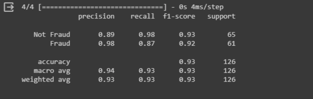

The classification report indicates that the model performs well in identifying both "Not Fraud" and "Fraud" transactions. It achieves high precision and recall for both classes, with an overall accuracy of 93%.

This suggests that the model makes accurate predictions and effectively distinguishes between fraudulent and non-fraudulent transactions.

Saving the Model

To deploy the model in real-world applications, it needs to be saved and integrated into existing fraud detection systems, ensuring seamless operation and reliability.

shallow_nn.save("shallow_nn_b_model.h5")

Future Trends

Graph Analytics: Integration of graph analytics techniques to analyze complex networks of relationships between entities, such as customers, merchants, and transactions. Graph-based approaches, combined with machine learning, can identify patterns of fraudulent behavior that are not apparent in traditional transaction data, enhancing fraud detection capabilities.

Explainable AI: Development of explainable AI (XAI) techniques to enhance transparency and interpretability of machine learning models. XAI methods help regulators and auditors, to understand how fraud detection models make decisions and identify potential biases or errors.

Federated Learning: Implementation of federated learning techniques to train machine learning models across distributed data sources while preserving data privacy. Federated learning enables collaboration between multiple institutions to collectively improve fraud detection models without sharing sensitive data.

Conclusion

In conclusion, while credit card fraud remains a persistent threat, the ongoing advancements in machine learning offer hope for more robust and effective fraud detection solutions in the future.

Frequently Asked Questions

How machine learning is used in credit card fraud detection?

Machine learning is employed in credit card fraud detection to analyze large volumes of transaction data and identify patterns indicative of fraudulent activity, enabling financial institutions to flag suspicious transactions in real-time.

What is credit card fraud detection model?

A credit card fraud detection model is a machine learning algorithm trained on historical transaction data to identify patterns indicative of fraudulent activity. These models utilize features such as transaction amount, location, and frequency to classify transactions as either fraudulent or legitimate.