3D scene flow: a complete guide on its application in self-driving cars

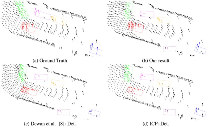
Table of Contents

1. Introduction
2. Various Methods for Obtaining 3D Scene Flow
3. Conclusion

Humans have been trying to develop self-driving cars for a long time. Thanks to the fast growing technology, recent years have witnessed enormous progress in Artificial Intelligence (AI) related fields such as computer vision, machine learning, and autonomous vehicles.

We humans, can seamlessly incorporate motion and depth information from our surroundings and that too at a very fast speed. We can estimate the motion of objects around us and judge in what direction they are moving. We can easily identify which objects are closer to us and which are farther. Many autonomous driving tasks, such as the 3D segmentation of moving objects, require this type of reasoning.

To drive better than humans, autonomous vehicles must first see better than humans. Building reliable vision capabilities for self-driving cars has been a major development hurdle. By combining a variety of sensors and using the modern day available technologies, however, developers have been able to create a detection system that can see a vehicle’s environment even better than human eyesight. 3D Scene flow is also a step in this direction. It is a process using which we track an object across various 3D images. Below is an example of the same.

Introduction

3D scene flow is the three-dimensional motion field of points across multiple 3D images (or 3D point clouds) just like optical flow is the motion of individual pixels across multiple 2D images (frames).

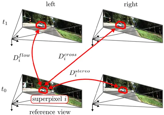
Two sequential stereo image pairs form the bare minimum setup for image-based scene flow estimate. By establishing correspondences between the four images, it is possible to fully characterize the 3D mobility of the surface point by determining its 3D location in both frames.

This information can then be utilized to judge the direction and velocity of movement of the object we are tracking, which might be a vehicle or a pedestrian or something else.

Before discussing more about 3D Scene Flow, let’s try to understand what is stereo imaging and optical flow first, as they are very important for obtaining 3D scene flow.

What is Stereo Imaging?

Stereo estimation is the process of extracting 3D information from 2D images captured by stereo cameras. This technique is used for creating or enhancing the illusion that an image has depth by using two slightly offset images. In the image below, you can see a stereo camera setup on the left with two cameras placed at some distance on a fixed rig and a pair of stereo images on the right, where one image is captured from the left camera and the other one is captured from the right camera at the same time.

In particular, stereo algorithms estimate depth information by finding correspondences between two images taken at the same point in time, typically by two cameras mounted next to each other on a fixed rig. So, a stereo-pair image contains two views of a scene side by side. One of the views is intended for the left eye and the other for the right eye. Both images are of the same scene or object but from a slightly different angle or perspective.

What is Optical Flow?

Optical flow is used to track the movement of an object in different frames, and this is generally achieved by tracking the movement of pixels associated with the object using displacement vectors. A displacement vector is used to specify the position of a certain object at any given point of time. Knowing the position of an object is vital when describing the motion of that body.

Most methods that compute optical flow assume that the color/intensity of a pixel is not changing as we move from one video frame to the next. But, in practice, computation of optical flow is susceptible to noise and illumination changes.

Optical flow not only helps identify which regions of the image are undergoing motion but also the velocity of motion. So, it can be used to detect and track vehicles in an automated traffic surveillance application as well.

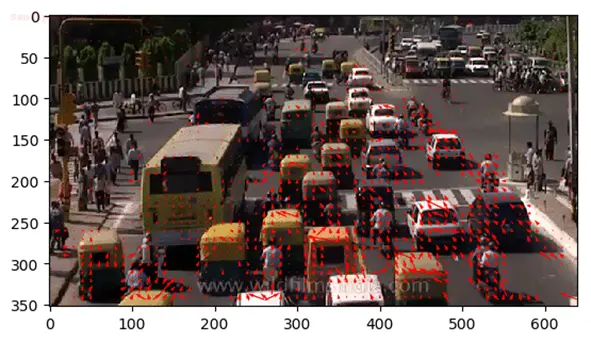
The image below is an example of the same. You can see the sparse optical flow of a traffic scene, where each arrow points in the direction of the predicted flow of the corresponding pixel.

Now, since we know the objective of 3D scene flow and we are also aware of the basics of stereo images (which serves as an input for various 3d scene flow methods) and optical flow (which is the 2d equivalent of 3d scene flow), let’s discuss about the various approaches that have been utilized to obtain 3d scene flow.

Various methods for obtaining 3D Scene Flow

There are mainly 3 types of approaches that have been utilized for obtaining the 3D scene flow. We have discussed them below.

1. Variational Methods

Traditionally, variational methods were used for obtaining 3D Scene Flow. This method uses several mathematical functions to detect and track pixels across various frames. Generally, an energy function is calculated that assigns low energies to the correct values and higher energies to the incorrect values.

Then a loss function is used to identify and reduce the higher energy values, or to bring the incorrect values closer to corresponding correct values.

In other words, two assumptions are characteristic for many variational optic flow methods: a brightness constancy assumption (where brightness is assumed constant over multiple frames) and a smoothness assumption (where a smoothness term is introduced as a prior).

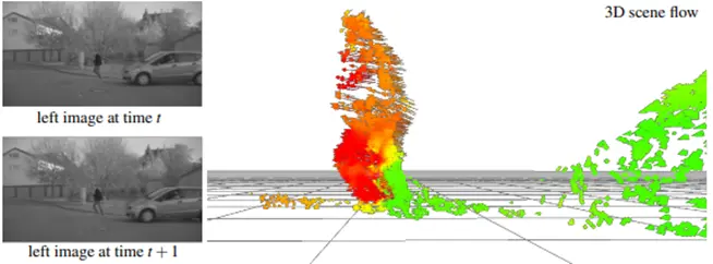
One such method was proposed by Wedel and his team where they presented a variational framework for estimating 3D scene flow using Stereo Images. Below is an example of the scene flow motion field they obtained. On the left you can see the image for two time instances. On the right is the obtained 3D scene flow, where you can see the moving person. The color encodes speed from stationary (green) to rapidly moving (red).

But such methods are generally very slow and the accuracy is also not very good, so they cannot be applied in applications such as self-driving cars where real-time and accurate processing is required.

However, assuming the scene as a collection of rigidly moving planar sections can help improve the performance of 3D Scene Flow models. More about this has been discussed in the further approaches.

2. Piecewise Rigidity Methods using Semantic Segmentation

In the piecewise rigidity methods, the scene is divided into various planes or objects. Each object is assumed to be a rigid pair of pixels, often called superpixels. By doing this, it becomes easier to track a pixel across various frames as a pixel associated with one object in one frame is most likely to be associated with the same object in the next frame. So, by detecting the object in the next frame we can easily track the pixels associated with it. For instance, in the case of automobiles in an autonomous driving scenario, a vehicle instance in one frame should have its pixels mapped to the same vehicle instance in the next frame.

Generally, semantic segmentation is used for detecting objects and pixels associated with it. The goal of semantic image segmentation is to label each pixel of an image with a corresponding class of what is being represented, as shown in the image below. Because we're predicting for every pixel in the image, this task is commonly referred to as dense prediction. Using semantic knowledge, we can limit the space of potential rigid body motions as segmented pixels that are grouped together are likely to move as a single object.

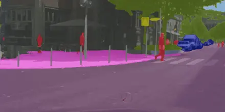
Various works have been done in this direction, some of them have been discussed below:

• Vogel and his team tried to achieve this by segmenting the image into separate regions to estimate the characteristics of each region's motion and shape. They employed a discrete optimization framework and their methodology greatly enhanced accuracy. You can see a glimpse of the results they obtained in the image below.

• Meanwhile, Lv and his team concentrated more on a productive solution to the issue using the same representation. For quicker inference, they carried out continuous optimization under the assumption of a fixed superpixel segmentation.
• Behl and his team examined the effects of instance segmentation, bounding box detection and 3D object coordinates on scene flow estimates and demonstrated which one is best for scene flow. They use the proposal-based instance segmentation method to get the bounding boxes and instance segmentation. 3D object coordinates are predicted using a Convolutional Neural Network (CNN) that was trained on 2D instance segmentations. The image below is a visual representation of the flow of their model.

• Ma and team have recently used a variety of inputs, including CNNs, to address the scene flow issue, such as Mask R-CNN for segmentation, PWC-Net for optical flow, and PSM-Net for stereo. They can train the entire pipeline end-to-end which helps improve the speed of the algorithm.

The use of semantic segmentation and piecewise rigidity assumption for 3D scene flow has helped achieve great improvements in accuracy as well as speed, making such methods the current state of the art. But these rigidity assumptions are very strong assumptions and in the real world are frequently broken by objects like bicycles, pedestrians and vegetation, which are made of various moving parts having complex motions. Although, treating each part as a separate superpixel might help.

The image-based algorithms calculate scene flow based on two successive image pairs taken by a calibrated stereo camera rig. However, the "curse of two-view geometry" affects stereo-based scene flow techniques, which means the depth inaccuracy increases quadratically with distance from the observer. To overcome this, various approaches have been proposed to calculate 3D scene flow directly from the 3D point clouds obtained from sensors like LiDARs.

3. Scene Flow from 3D Points

Point clouds are a collection of millions or billions of individual measurement points from the surface of objects represented in a 3D space. They are used to represent the 3D shape of the object. They can be acquired by laser scanners, drones or 3D cameras. Below is an example of the same.

The LiDAR (Light Detection and Ranging) technology is used by the majority of existing systems for self-driving cars to perceive 3D geometry. Laser scanners do not exhibit the stereo camera's quadratic error characteristic, in contrast to cameras. Laser scanners are also largely unaffected by lighting conditions and offer a 360-degree field of view with just one sensor.

A number of approaches have recently been put out for estimating 3D scene flow from pairs of unstructured 3D point clouds, like:

• One such method is given by Dewan and his team. Their method uses a variational approach over 3D point clouds. So, they formulate the problem as an energy minimization problem, where they assume local geometric constancy and incorporate regularization for smooth motion fields. However, their method fails to perform in the presence of unclear or noisy inputs.
• Behl and team propose another similar method where they use CNNs as a general end-to-end trainable model to tackle the scene flow issue. However, the majority of the available area is empty due to the sparse nature of the LiDAR data, which makes the method memory and computationally inefficient.

Conclusion

A key characteristic of dynamic scenes is the flow of the scene in three dimensions, which plays a critical role in tracking the movement of objects in the scene.

But, several challenges make this task very difficult, like partially occluded objects or illumination changes across frames. Due to matching issues and the autonomous motion of cars, car surfaces are one of the most challenging areas in 3D Scene Flow. Another frequent source of error are pixels that are close to the image or object boundary, particularly on the road surfaces in front of the car where significant changes take place.

Although the difficulty is mitigated by the local planarity and rigidity assumptions. Either the assumption of rigidly moving segments or semantic cues are used by all top-performing models, but these assumptions are frequently broken by complicated geometric objects like bicycles, pedestrians, and vegetation. In contrast, since non-rigid objects can be described by many superpixels, segmenting the scene into superpixels solves this issue and improves speed.

Semantic image understanding, by segmenting instances of cars, appears to be a feasible approach, especially at the object level. Such methods are the current state of the art. To gather this data, however, a separate network must be trained, and prediction errors can result in flaws in the final scene flow estimation.

CNN based methods give fast and accurate outputs once trained, but need a lot of data to be trained on. Currently, only few datasets are available for scene flow. The KITTI scene flow benchmark is the most prominent dataset allowing the comparison of algorithms on an online evaluation server. But, since KITTI is too small for deep learning, the Flying Things dataset is frequently used for pre-training.

The challenge of establishing a reliable, precise and real-time multi-frame scene flow estimate still remains an open problem and requires further work.

With all the advances in technology, we have come a long way from when we started developing the first self-driving cars, but we still have a long way to go. It will take at least a decade before self-driving cars hit the highways, but for fully self-driving vehicles, we will probably need to wait several more years.